In this article, first briefly explain what the mixed density network (MDN) is, then build the MDN model using Python code, and finally use the built model for multiple regression and test the effect.

regression

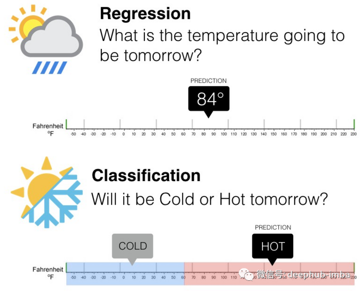
"Regression prediction modeling is to approximate the mapping function (f) from input variable (X) to continuous output variable (y) [...] Regression problems need to predict specific values. Problems with multiple input variables are often referred to as multiple regression problems. For example, predicting the value of a house may be between $100000 and $200000

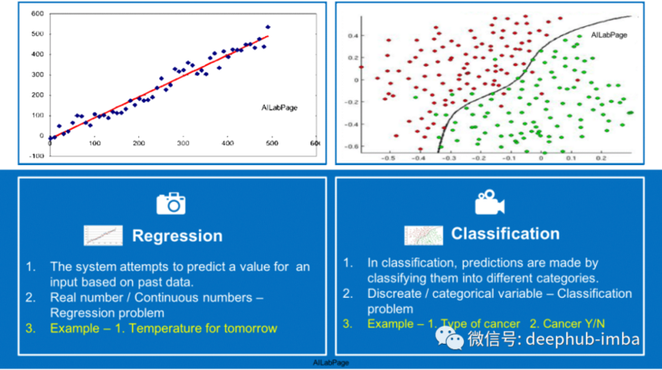
This is another visual explanation to distinguish between classification problem and regression problem, as follows:

Another example

density

What does DENSITY mean? This is a quick, popular example:

Suppose pizza is being delivered for pizza hut. Now record the time (in minutes) of each delivery just made. After 1000 deliveries, visualize the data to see how the work is performing. This is the result:

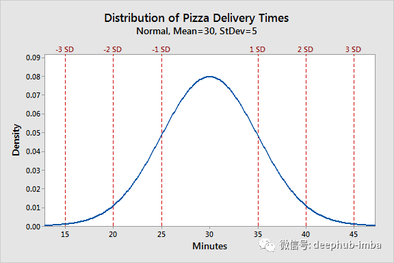
This is the "density" of pizza delivery time data distribution. On average, each delivery takes 30 minutes (peak in the figure). It also said that in 95% of cases (2 standard deviations 2sd), delivery takes 20 to 40 minutes to complete. The density category represents the "frequency" of the time result. The difference between "frequency" and "density" is:

·Frequency: if you draw a histogram under this curve and count all bin s, it will sum to any integer (depending on the total number of observations captured in the dataset).

·Density: if you draw a histogram under this curve and calculate all bin, it will sum to 1. We can also call this curve probability density function (pdf).

In statistical terms, this is a beautiful normal / Gaussian distribution. This normal distribution has two parameters:

mean value

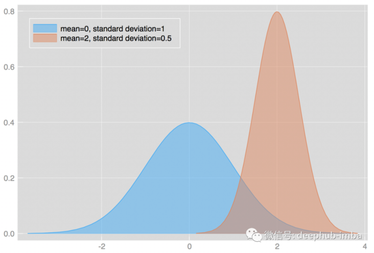
·Standard deviation: "a standard deviation is a number that describes how a set of measurements is expanded from the average (average) or expected value. A low standard deviation means that most numbers are close to the average. A high standard deviation means that the numbers are more dispersed“

The change of mean and standard deviation will affect the shape of distribution. For example:

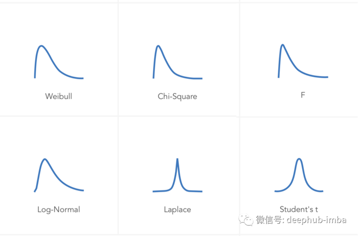
There are many different distribution types with different types of parameters. For example:

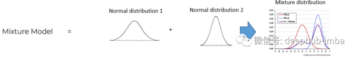
Mixed density

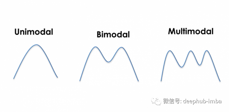
Now let's look at these three distributions:

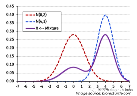
If we use this bimodal distribution (also known as the general distribution):

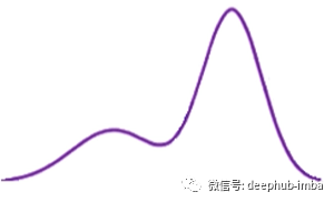
The mixed density network uses the assumption that any general distribution like this bimodal distribution can be decomposed into a mixture of normal distribution (the mixture can also be customized with other types of distribution, such as Laplace):

Network architecture

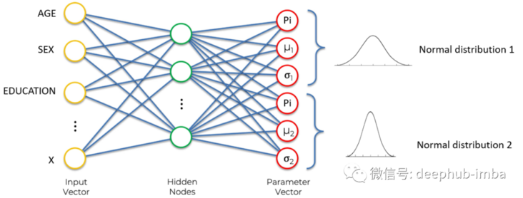
Hybrid density network is also an artificial neural network. This is a classic example of a neural network:

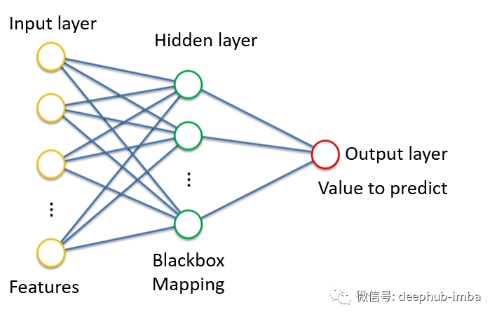
Input layer (yellow), hidden layer (green), and output layer (red).

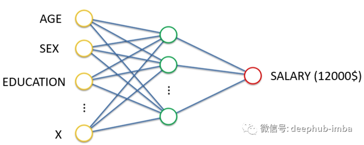
If we define the goal of neural network as learning to output continuous values given some input characteristics. In the above example, given age, gender, education and other characteristics, the neural network can perform regression.

Density network

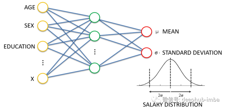
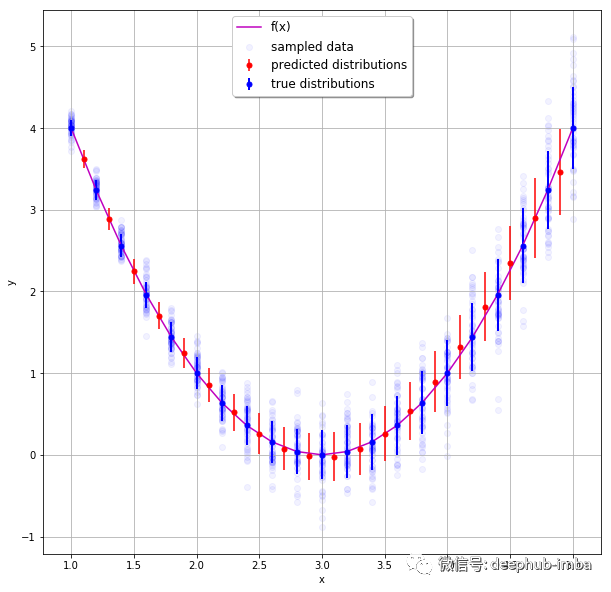
Density network is also a neural network. Its goal is not to simply learn to output a single continuous value, but to learn to output distribution parameters (here mean and standard deviation) given some input characteristics. In the above example, given the characteristics of age, gender and education, neural network learning predicts the mean and standard deviation of the expected wage distribution. Prediction distribution has many advantages over predicting a single value, for example, it can give the uncertainty boundary of prediction. This is the "Bayesian" method to solve the regression problem. The following is a good example of predicting the distribution of each expected continuous value:

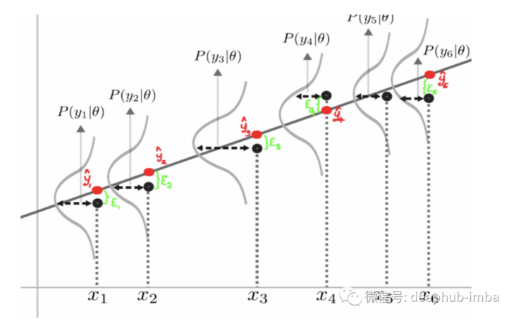
The following picture shows us the expected value distribution of each prediction instance:

Mixed density network

Finally, back to the point, the goal of hybrid density network is to learn the parameters of all distributions (here mean, standard deviation and PI) mixed in the general distribution under the condition of given specific input characteristics. The new parameter "Pi" is the mixing parameter, which gives the weight / probability of a given distribution in the final mixing.

The final results are as follows:

Example 1: MDN class of univariate data

The above definition and theoretical basis have been introduced. Now let's start the code demonstration:

import numpy as np
import pandas as pd

from mdn_model import MDN

from sklearn.datasets import make_moons
from sklearn.preprocessing import StandardScaler
import matplotlib.pyplot as plt
import seaborn as sns

from sklearn.linear_model import LinearRegression
from sklearn.kernel_ridge import KernelRidge

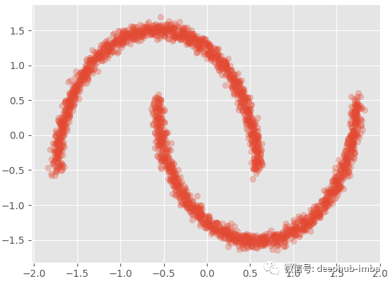
plt.style.use('ggplot')

Generate the famous "half moon" dataset:

X, y = make_moons(n_samples=2500, noise=0.03)
y = X[:, 1].reshape(-1,1)
X = X[:, 0].reshape(-1,1)

x_scaler = StandardScaler()
y_scaler = StandardScaler()

X = x_scaler.fit_transform(X)
y = y_scaler.fit_transform(y)

plt.scatter(X, y, alpha = 0.3)

Plot the density distribution of the target value (y):

sns.kdeplot(y.ravel(), shade=True)

By viewing the data, we can see that there are two overlapping clusters:

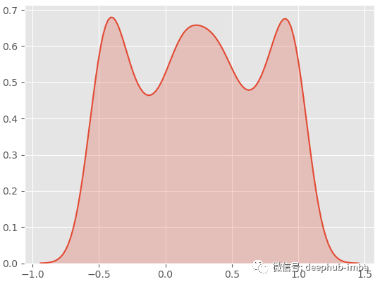
This is a good multimodal distribution (general distribution). If we try a standard linear regression on this data set to predict y with X:

model = LinearRegression()
model.fit(X.reshape(-1,1), y.reshape(-1,1))
y_pred = model.predict(X.reshape(-1,1))

plt.scatter(X, y, alpha = 0.3)
plt.scatter(X,y_pred)
plt.title('Linear Regression')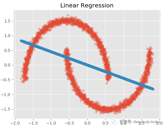

sns.kdeplot(y_pred.ravel(), shade=True, alpha = 0.15, label = 'Linear Pred dist')      
sns.kdeplot(y.ravel(), shade=True, label = 'True dist')

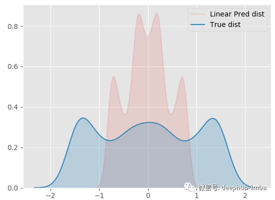
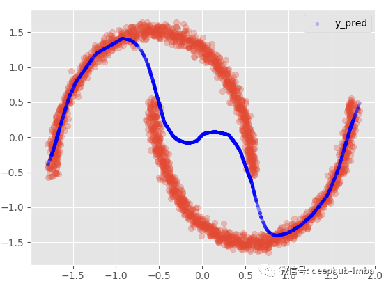
The effect must be bad! Now let's try a nonlinear model (radial basis function kernel ridge regression):

model = KernelRidge(kernel = 'rbf')
model.fit(X, y)
y_pred = model.predict(X)


plt.scatter(X, y, alpha = 0.3)
plt.scatter(X,y_pred)
plt.title('Non Linear Regression')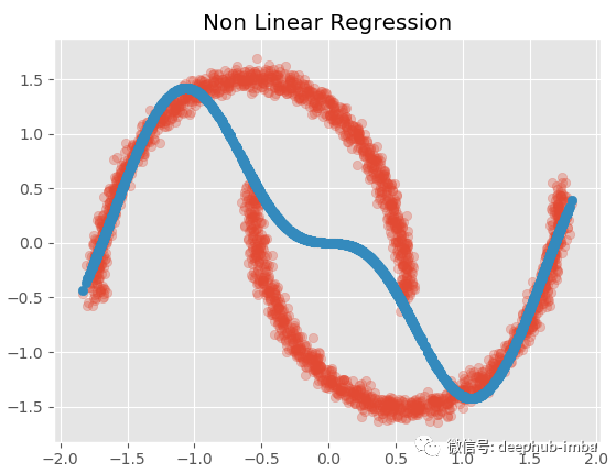

sns.kdeplot(y_pred.ravel(), shade=True, alpha = 0.15, label = 'NonLinear Pred dist')      
sns.kdeplot(y.ravel(), shade=True, label = 'True dist')

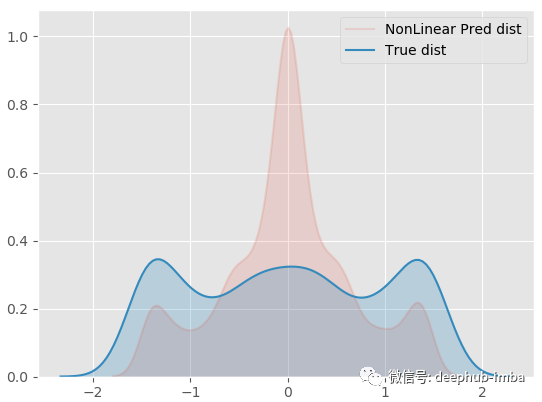
Although the result is not satisfactory, it is much better than the above linear regression.

The main reason for the failure of both models is that there are multiple different Y values for the same x value... More specifically, there seems to be more than one possible y distribution for the same X. The regression model only tries to find the optimal function to minimize the error, and does not take into account the mixing of density. Therefore, those X in the middle have no unique y solution. They have two possible solutions, which leads to the above problems.

Now let's try an MDN model. Here we have implemented a fast and easy-to-use "fit predict" and "sklearn like" custom python MDN class. If you want to use it yourself, this is a link to python code (please note: This MDN class is experimental and has not been widely tested): https://github.com/CoteDave/b...

In order to be able to use this class, there are sklearn, tensorflow probability, tensorflow < 2, umap and hdbscan (used to customize the visualization class function).

EPOCHS = 10000
BATCH_SIZE=len(X)

model = MDN(n_mixtures = -1, 
            dist = 'laplace',
            input_neurons = 1000, 
            hidden_neurons = [25], 
            gmm_boost = False,
            optimizer = 'adam',
            learning_rate = 0.001, 
            early_stopping = 250,
            tf_mixture_family = True,
            input_activation = 'relu',
            hidden_activation = 'leaky_relu')

model.fit(X, y, epochs = EPOCHS, batch_size = BATCH_SIZE)

The parameters of class are summarized as follows:

· n_ Mixes: the number of distribution mixes used by the MDN. If set to - 1, it will "automatically" find the best number of blends using Gaussian mixture model (GMM) and HDBSCAN model on X and y.

·dist: the type of distribution used in mixing. At present, there are two options; "Normal" or "Laplace". (based on some experiments, Laplace distribution has better results than normal distribution).

· input_neurons: the number of neurons used in the input layer of MDN

· hidden_neurons: hidden layer architecture of MDN. A list of neurons for each hidden layer. This parameter enables you to select the number of hidden layers and the number of neurons per hidden layer.

· gmm_boost: Boolean value. If set to True, cluster features are added to the dataset.

·optimizer: the optimization algorithm to use.

· learning_rate: learning rate of optimization algorithm

· early_stopping: avoid over fitting during training. This trigger determines when to stop training when the indicator has not changed in a given number of periods.

· tf_mixture_family: Boolean value. If set to True, TF is used_ Mix series (recommended): mix objects realize batch mixed distribution.

· input_activation: the activation function of the input layer

· hidden_activation: activation function of hidden layer

Now the MDN model has fitted the data, sampled from the mixed density distribution and plotted the probability density function:

model.plot_distribution_fit(n_samples_batch = 1)

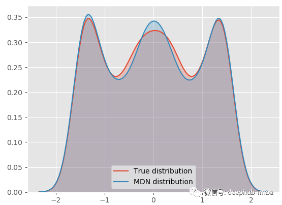
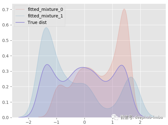
Our MDN model is very suitable for real general distribution! Let's decompose the final mixed distribution into each distribution and see what it looks like:

model.plot_all_distribution_fit(n_samples_batch = 1)

Use the learned mixed distribution to sample some Y data again, and compare the generated sample with the real sample:

model.plot_samples_vs_true(X, y, alpha = 0.2)

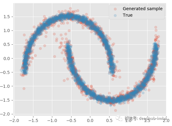
It is very close to the actual data. If X is given, multiple batches of samples can be generated to generate quantile, mean and other statistical information:

generated_samples = model.sample_from_mixture(X, n_samples_batch = 10)
generated_samples

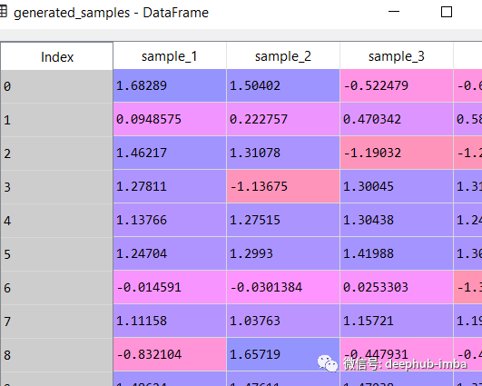
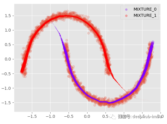
Plot the average of each learning distribution and their respective blend weights (pi):

plt.scatter(X, y, alpha = 0.2)
model.plot_predict_dist(X, with_weights = True, size = 250)

With the mean and standard deviation of each distribution, it can also be plotted with complete uncertainty; Suppose we plot the mean with a 95% confidence interval:

plt.scatter(X, y, alpha = 0.2)
model.plot_predict_dist(X, q = 0.95, with_weights = False)

Mix the distributions together. When there are multiple y distributions for the same X, we use the highest Pi parameter value to select the most likely mixture:

Y_preds = for each X, select the y-means of the distribution with the maximum probability / weight (Pi parameter)

plt.scatter(X, y, alpha = 0.3)
model.plot_predict_best(X)

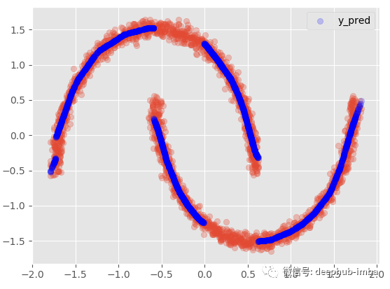
This method is not ideal, because there are obviously two different clusters overlapping in the data, and the density is almost equal. So that the error will be higher than the standard regression model. This also means that there may be a lack of important features in the dataset that can help avoid clusters overlapping in higher dimensions.

We can also choose to use the Pi parameter and the mean mixed distribution of all distributions:

· Y_preds = (mean_1 Pi1) + (mean_2 Pi2)

plt.scatter(X, y, alpha = 0.3)
model.plot_predict_mixed(X)

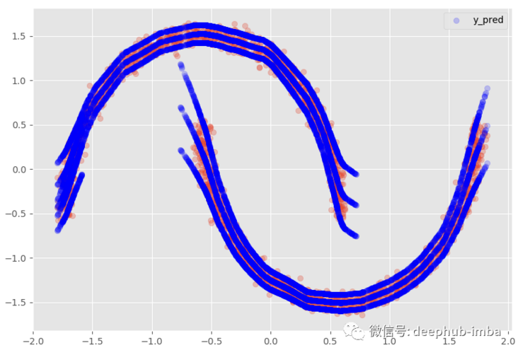
If we add 95 confidence intervals:

This option provides almost the same results as the nonlinear regression model, mixing everything to minimize the distance between points and functions. In this very special case, my favorite choice is to assume that in some areas of the data, X has multiple Y, while in other areas; Use only one of these blends.:

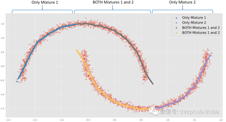
For example, when X = 0, each blend may have two different Y solutions. When X = -1.5, there is a unique y solution in mix 1. According to the use case or business context, when there are multiple solutions in the same X, actions or decisions can be triggered.

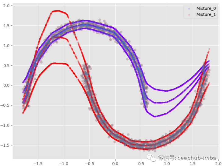
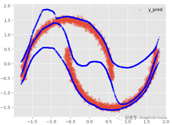
The meaning of this option is that when there is overlapping distribution (if both mixing probabilities are > = given probability threshold), the line will be copied:

plt.scatter(X, y, alpha = 0.3)
model.plot_predict_with_overlaps(X)

95% confidence interval:

The data set row increased from 2500 to 4063, and the final forecast data set is as follows:

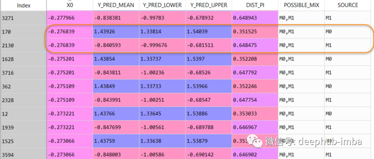
In this data table, when X = -0.276839, Y can be 1.43926 (the probability of mixed \ _0is 0.351525), but it can also be -0.840593 (the probability of mixed \ _1is 0.648475).

Instances with multiple distributions also provide important information that something is happening in the data and may require more analysis. It may be some data quality problems, or it may indicate the lack of an important feature in the data set!

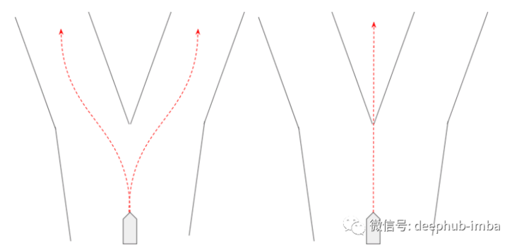
"Traffic scene prediction is a good example of using a mixed density network. In traffic scene prediction, we need a behavior distribution that can be displayed - for example, an agent can turn left, right or straight. Therefore, the mixed density network can be used to represent the" behavior "in each mixture it learns, The behavior is composed of probability and trajectory ((x, y) coordinates are in a certain time range in the future).

Example 2: multivariate regression with MDN

Finally, does MDN perform well on multiple regression?

We will use the following data sets:

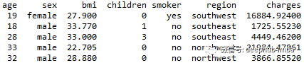
·Age: the age of the primary beneficiary

·Gender: Insurance contractor gender, female, male

·bmi: body mass index, which provides an understanding of the body. Relative to the weight of relatively high or low height, the objective weight index (kg / m ^ 2) of the ratio of height to weight is used, which is ideally 18.5 to 24.9

·Children: number of children covered by health insurance / number of dependants

·Smoker: smoking

·Region: the beneficiary's residential area in the United States, northeast, Southeast, southwest and northwest.

·Expenses: personal medical expenses charged by health insurance. This is the goal we want to predict

The question statement is: can you accurately predict the insurance cost (charge)?

Now let's import the dataset:

"""
#################
# 2-IMPORT DATA #
#################
"""
dataset = pd.read_csv('insurance_clean.csv', sep = ';')

##### BASIC FEATURE ENGINEERING
dataset['age2'] = dataset['age'] * dataset['age']
dataset['BMI30'] = np.where(dataset['bmi'] > 30, 1, 0)
dataset['BMI30_SMOKER'] = np.where((dataset['bmi'] > 30) & (dataset['smoker_yes'] == 1), 1, 0)
"""
######################
# 3-DATA PREPARATION #
######################
"""
###### SPLIT TRAIN TEST
from sklearn.model_selection import train_test_split
X = dataset[dataset.columns.difference(['charges'])]
y = dataset[['charges']]

X_train, X_test, y_train, y_test = train_test_split(X, y, 
                                                    test_size=0.25, 
                                                    stratify = X['smoker_yes'], 
                                                    random_state=0)


test_index = y_test.index.values
train_index = y_train.index.values
features = X.columns.tolist()

##### FEATURE SCALING 
from sklearn.preprocessing import StandardScaler
x_scaler = StandardScaler()
y_scaler = StandardScaler()

X_train = x_scaler.fit_transform(X_train)
#X_calib = x_scaler.transform(X_calib)
X_test = x_scaler.transform(X_test)

y_train = y_scaler.fit_transform(y_train)
#y_calib = y_scaler.transform(y_calib)
y_test = y_scaler.transform(y_test)

y_test_scaled = y_test.copy()

The data is ready for training

EPOCHS = 10000
BATCH_SIZE=len(X_train)

model = MDN(n_mixtures = -1, #-1
            dist = 'laplace',
            input_neurons = 1000, #1000
            hidden_neurons = [], #25
            gmm_boost = False,
            optimizer = 'adam',
            learning_rate = 0.0001, #0.00001
            early_stopping = 200,
            tf_mixture_family = True,
            input_activation = 'relu',
            hidden_activation = 'leaky_relu')

model.fit(X_train, y_train, epochs = EPOCHS, batch_size = BATCH_SIZE)

After the training, use the "best mixing probability (Pi parameter) strategy" to predict the test data set and draw the results (y_pred vs y_test):

y_pred = model.predict_best(X_test, q = 0.95, y_scaler = y_scaler)
model.plot_pred_fit(y_pred, y_test, y_scaler = y_scaler)

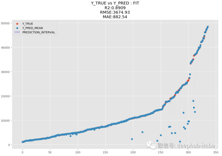
model.plot_pred_vs_true(y_pred, y_test, y_scaler = y_scaler)

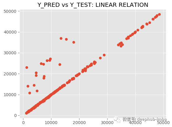
R2 is 89.09 and MAE is 882.54. MDN is great. Let's draw a graph of fitting distribution and real distribution for comparison:

model.plot_distribution_fit(n_samples_batch = 1)

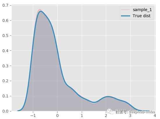
Almost as like as two peas! Decompose the hybrid model to see what happens:

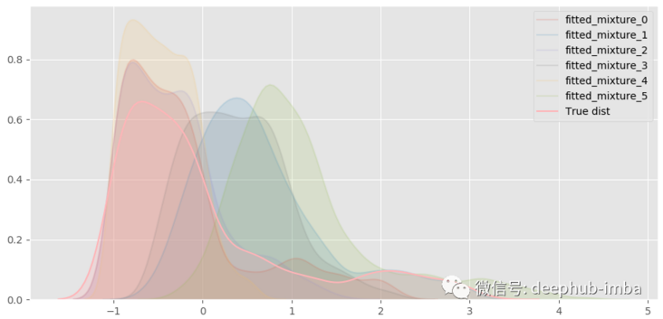
A total of six different distributions were mixed.

Generate multivariable samples from the fitted mixed model (apply PCA to visualize the results in 2D):

model.plot_samples_vs_true(X_test, y_test, alpha = 0.35, y_scaler = y_scaler)

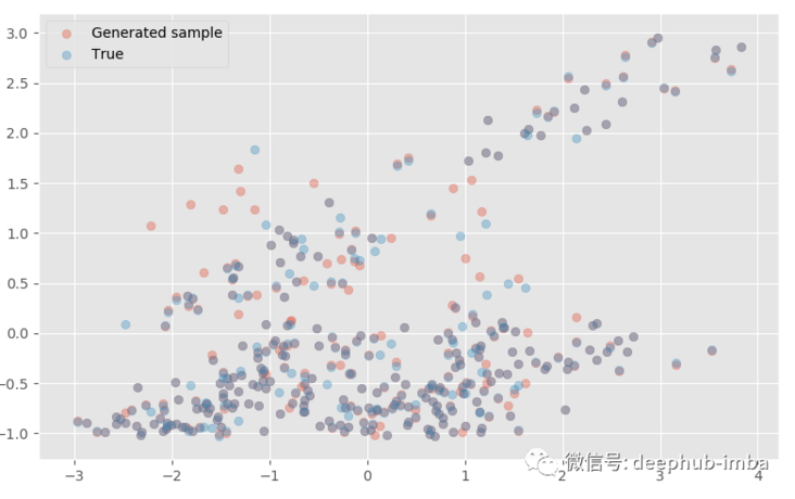
The generated sample is very close to the real sample! If we wish, we can also make predictions from each distribution:

y_pred_dist = model.predict_dist(X_test, q = 0.95, y_scaler = y_scaler)
y_pred_dist

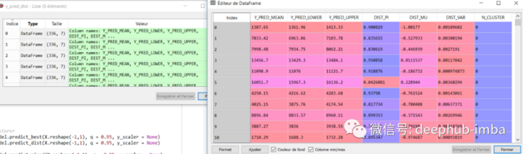
summary

·Compared with linear or nonlinear classical ML models, MDN performs well in univariate regression data sets, where two clusters overlap each other, and X may have multiple Y outputs.

·MDN is also good at multiple regression, and can compete with popular models such as XGBoost

·MDN is an excellent and unique tool in ML, which can solve specific problems that cannot be solved by other models (learning from data obtained from mixed distribution)

·With the MDN learning distribution, the uncertainty can also be calculated by prediction or new samples can be generated from the learning distribution

There are many codes in this article. Here is a complete notebook, which can be downloaded and run directly:

https://www.overfit.cn/post/20245a8446ae43e3982b48e4320991ab

Author: Dave Cote, M.Sc