1. Mean square error of single measurement and mean square error of arithmetic mean

array = [
  120.0360
  120.0390
  120.0260
  120.0270
  120.0350
  120.0360
  120.0310
  120.0250
  119.9830
  120.0410];
average = mean(array);
r = array - average;
error1 = (sum(r.^2)/(size(array,1)-1))^(1/2);%Mean square error of single measurement
error2 = error1/size(array,1)^(1/2);%Mean square error of arithmetic mean
disp(average);
disp(error1);
disp(error2);

  120.0279

    0.0167

    0.0053

2. Weighted calculation of the most probable value

average_array = [
    36
    42
    33];
error_array = [
    0.7000
    1.2000
    0.7000];
average = sum(average_array.*error_array)/sum(error_array);%Weighted most probable value
disp(average);

   37.9615

3. Error transfer function

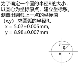
syms x y real;
f(x,y) = (x^2 + y^2)^(1/2);
df_array = [
    diff(f,x)
    diff(f,y)];
delta_array = [
    0.0050
    0.0070];
x = 5.02;
y = 8.98;
R = eval(f);
error = sum((eval(df_array).*delta_array).^2).^(1/2);%Law of error propagation
disp(R);
disp(error);

   10.2879

    0.0066

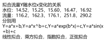
4. Function fitting

Source: https://www.cnblogs.com/yabin/p/6417566.html

History error code 1

% Independent variable and dependent variable
x = [
14.5200
15.2500
15.6000
16.4700
16.9200];
Y = [
116.2000
162.3000
176.1000
251.8000
290.2000];

% The fitted function is used for fit function
linearFun1 = 'a*x+b';
powerFun1 = 'a*x^b+c';
indexFun1 = 'a*exp(b*x)+c';
sinFun1 = 'a*sin(x+b)+c';
Fun1_array = {
linearFun1
powerFun1
indexFun1
sinFun1};
% The arguments of the fitted function are used for fit function
linearX1 = {'x'};
powerX1 = {'x'};
indexX1 = {'x'};
sinX1 = {'x'};
X1_array = {
linearX1
powerX1
indexX1
sinX1};
% The coefficients of the fitted function are used for fit function
linearCo1 = {'a','b'};
powerCo1 = {'a','b','c'};
indexCo1 = {'a','b','c'};
sinCo1 = {'a','b','c'};
Co1_array = {
linearCo1
powerCo1
indexCo1
sinCo1};

% The fitted function is used for nlinfit function
linearFun2 = @(x,Co2) Co2(1).*x+Co2(2);
powerFun2 = @(x,Co2) Co2(1).*x.^Co2(2)+Co2(3);
indexFun2 = @(x,Co2) Co2(1).*exp(Co2(2).*x)+Co2(3);
sinFun2 = @(x,Co2) Co2(1).*sin(x+Co2(2))+Co2(3);
Fun2_array = {
linearFun2
powerFun2
indexFun2
sinFun2};

% Sets the starting search point for the coefficient
startPos = [1,1];

% Total number of functions to be fitted
length = size(Fun1_array,1);
% Fitting result array
% fitFunResult = zeros(size(Fun1_array));
% Co2Result = zeros(size(Fun1_array));

for i = 1:1:length
    subplot(length,1,i);
    string(Fun1_array(i))
    string(X1_array(i))
    Co1_array(i)
    % use fit Function fitting
    funType = fittype(string(Fun1_array(i)),'independent',string(X1_array(i)),'coefficients',Co1_array(i));
    opt = fitoptions(funType);
    set(opt,'StartPoint',startPos);
    fitFunResult(i) = fit(x,Y,funType,opt);
    % Print results
    disp(fitFunResult(i));
    % Draw a picture
    hold on;
    plot(fitFunResult(i),'r',x,Y,'*');
    % use nlinfit Function fitting 
    Co2Result(i) = nlinfit(x,Y,Fun2_array(i),startPos);
    % Print results
    disp('nlinfit The coefficient matrix after fitting is:');
    disp(Co2Result(i));
    % Draw a picture
    hold on;
    xmax = max(x);
    xmin = min(x);
    xnum = 2*length(x)+50;
    x = linspace(xmin,xmax,xnum);
    fun2 = Fun2_array(i);
    y = fun2(x,Co2Result(i));
    plot(x,y,'g');
    legend('raw data','fit fitting','nlinfit fitting');
end

Error alert:

Wrong use of cellstr (line 44)
Element 1 is not a string scalar or character array. All elements of cell input must be string scalar or character array.
　
Error: fittype > iassertvalidvariablenames (line 1053)
names = cellstr( names );
　
Error: fittype > isetvariablenames (line 1044)
iAssertValidVariableNames( variableName );
　
Error fittype > iparseparameters (line 561)
obj = iSetVariableNames( obj, 'coeff', value );
　
Error fittype > icreatecustomfittype (line 429)
obj = iParseParameters(obj,varargin(2:end));
　
Error fittype > icreatefitttype (line 353)
obj = iCreateCustomFittype( obj, varargin{:} );
　
Error fittype (line 330)
obj = iCreateFittype( obj, varargin{:} );

The main reason is that the transmission of characters is a little hard
I tried tostring, but it didn't work. I didn't want to hang myself from a tree

After that, I tried it. It seems that the cell array needs to use {} to extract data hhh

% Independent variable and dependent variable
x = [
14.5200
15.2500
15.6000
16.4700
16.9200];
Y = [
116.2000
162.3000
176.1000
251.8000
290.2000];

% The fitted function is used for nlinfit function
linearFun = @(x,Co2) Co2(1).*x+Co2(2);
powerFun = @(x,Co2) Co2(1).*x.^Co2(2)+Co2(3);
indexFun = @(x,Co2) Co2(1).*exp(Co2(2).*x)+Co2(3);
sinFun = @(x,Co2) Co2(1).*sin(x+Co2(2))+Co2(3);
Fun_array = {
linearFun
powerFun
indexFun
sinFun};

% Sets the starting search point for the coefficient
startPos = [1,1];

% Total number of functions to be fitted
length = size(Fun1_array,1);
% Fitting result array
% fitFunResult = zeros(size(Fun1_array));
% CoResult = zeros(size(Fun1_array));

for i = 1:1:length
    subplot(length,1,i);
    Fun_array{i}
    % use nlinfit Function fitting 
    CoResult(i) = nlinfit(x,Y,Fun_array{i},startPos);
    % Print results
    disp('nlinfit The coefficient matrix after fitting is:');
    disp(CoResult(i));
    % Draw a picture
    hold on;
    xmax = max(x);
    xmin = min(x);
    xnum = 2*length(x)+50;
    x = linspace(xmin,xmax,xnum);
    Fun = Fun_array(i);
    y = Fun(x,CoResult(i));
    plot(x,y,'g');
end

Error warning:

Incorrect use of nlinfit (line 219)
MODELFUN must be a function that returns a fitted value vector of the same size as Y (5-by-1). The model function you provided returns the result 1-by-2.
　
One of the common reasons for size mismatches is to use matrix operators (*, /,) in functions instead of the corresponding element operators (. *,. /,.).

Then I changed it according to this

% The fitted function is used for nlinfit function
linearFun = @(x,Co) Co(1)*x+Co(2);
powerFun = @(x,Co) Co(1)*x^Co(2)+Co(3);
indexFun = @(x,Co) Co(1)*exp(Co(2)*x)+Co(3);
sinFun = @(x,Co) Co(1)*sin(x+Co(2))+Co(3);

I changed it to this or not

I feel like I'm no different from the official example
Well, maybe the parameter needs to be placed in front of the parameter list

Change it to this. Put it in the front

% The fitted function is used for nlinfit function
linearFun = @(Co,x) Co(1)*x+Co(2);
powerFun = @(Co,x) Co(1)*x^Co(2)+Co(3);
indexFun = @(Co,x) Co(1)*exp(Co(2)*x)+Co(3);
sinFun = @(Co,x) Co(1)*sin(x+Co(2))+Co(3);

It's ok now, but, uh, rank loss
Maybe I chose the wrong starting point

Well, after the experiment, blindly choosing the starting point will directly jam hhh, which should never converge

It's over. In fact, as a cycle, there is no universality at all. It's better to write alone hhh

clc;

% Independent variable and dependent variable
x = [
14.5200
15.2500
15.6000
16.4700
16.9200];
Y = [
116.2000
162.3000
176.1000
251.8000
290.2000];

% The fitted function is used for nlinfit function
linearFun = @(Co,x) Co(1)*x+Co(2);
powerFun = @(Co,x) Co(1)*x^Co(2)+Co(3);
indexFun = @(Co,x) Co(1)*exp(Co(2)*x)+Co(3);
sinFun = @(Co,x) Co(1)*sin(x+Co(2))+Co(3);
Fun_array = {
linearFun
powerFun
indexFun
sinFun};

% Sets the starting search point for the coefficient
startPos = {
    [50,-600]'
    [1,2,-100]'
    [2,0.25,50]'
    [100,0,-100]'};
    
% Total number of functions to be fitted
count = size(Fun_array,1);

for i = 1:1:count
    subplot(count,1,i);
    % use nlinfit Function fitting 
    CoResult = nlinfit(x,Y,Fun_array{i},startPos{i});
    % Print results
    disp('nlinfit The coefficient matrix after fitting is:');
    disp(CoResult);
    % Draw a picture
    hold on;
    xmax = max(x);
    xmin = min(x);
    xnum = 2*length(x)+50;
    x = linspace(xmin,xmax,xnum);
    Fun = Fun_array{i};
    y = Fun(CoResult,x);
    plot(x,y,'g');
end

Then simplify it. If you write it directly, there will be a power seeking error

Incorrect use of nlinfit (line 213)
Error calculating model function '@ (Co,x)Co(1)*x^Co(2)+Co(3)'.
　
reason:
Incorrect use ^ (line 51)
The dimension used to exponentiate the matrix is incorrect. Check that the matrix is square and the power is scalar. To perform > power by element matrix, use '. ^'.

If it is changed to. ^, Another error that does not allow ^ will appear

Incorrect use of nlinfit (line 219)
MODELFUN must be a function that returns a fitted value vector of the same size as Y (5-by-1). The model function you provided returns the result 1-by-60.
　
One of the common reasons for size mismatches is to use matrix operators (*, /,) in functions instead of the corresponding element operators (. *,. /,.).

Although his error message means that I can't use ^, when I change all operators to element operators, I still can't... I can't understand

Finally, I found that the variable names in my argument array and anonymous function handle are the same... xs

Code that can run normally:

clear;

% Independent variable and dependent variable
X = [
14.5200
15.2500
15.6000
16.4700
16.9200];
Y = [
116.2000
162.3000
176.1000
251.8000
290.2000];

% The fitted function is used for nlinfit function
linearFun = @(Co,x) Co(1).*x+Co(2);
powerFun = @(Co,x) Co(1).*x.^Co(2)+Co(3);
indexFun = @(Co,x) Co(1).*exp(Co(2).*x)+Co(3);
sinFun = @(Co,x) Co(1).*sin(x+Co(2))+Co(3);
Fun_array = {
linearFun
powerFun
indexFun
sinFun};

% Sets the starting search point for the coefficient
startPos = {
    [50,-600]'
    [1,2,-100]'
    [2,0.25,50]'
    [100,0,-100]'};
    
% Total number of functions to be fitted
count = size(Fun_array,1);

for i = 1:1:count
    subplot(count,1,i);
    % use nlinfit Function fitting 
    CoResult = nlinfit(X,Y,Fun_array{i},startPos{i});
    % Print results
    disp('nlinfit The coefficient matrix after fitting is:');
    disp(CoResult);
    % Draw a picture
    hold on;
    xmax = max(X);
    xmin = min(X);
    xnum = 2*length(X)+50;
    x = linspace(xmin,xmax,xnum);
    Fun = Fun_array{i};
    y = Fun(CoResult,x);
    plot(x,y,'g');
end

Output:

nlinfit The coefficient matrix after fitting is:
   73.0654
 -951.6060
 warning: Iteration limit exceeded. The result of the last iteration will be returned.
nlinfit The coefficient matrix after fitting is:
    0.0003
    4.9155
  -39.7506
nlinfit The coefficient matrix after fitting is:
    3.4509
    0.2749
  -70.1296
nlinfit The coefficient matrix after fitting is:
  -90.9788
   -0.2107
  209.3732

5. Moditu

Source: https://blog.csdn.net/PriceCheap/article/details/120975300

Re = 3:0.01:8;
epsilon = [0.0001 0.001 0.01 0.05];
for i=1:1:4
f = colebrook(10.^Re,epsilon(i)); 
plot(Re,f);
hold on
end
f2 = 64./(10.^Re);
hold on
plot(Re,f2);

6. Error line diagram

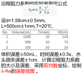
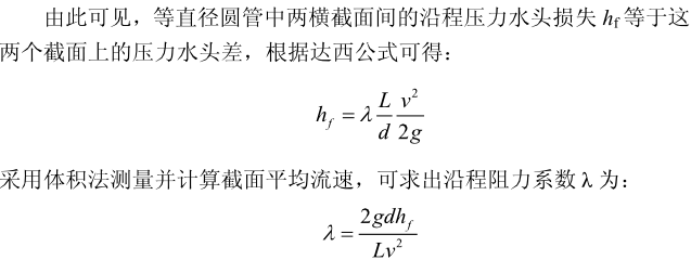
% hold v = V/S/t = 4*V/(pi*d^2*t) Substitute Darcy's formula and get
% lambda = pi*2*g*d^5*hf*t^2/(8*L*V^2)

clear;

syms d L V t hf real;
pi = 3.14;
g = 9.8;
lambda(d,L,V,t,hf) = pi*2*g*d^5*hf*t^2/(8*L*V^2);
dlambda_array = [
    diff(lambda,d)
    diff(lambda,L)
    diff(lambda,V)
    diff(lambda,t)
    diff(lambda,hf)];
delta_array = [
    0.5 * 1e-3
    1 * 1e-3
    50 * 1e-6
    0.5
    1 * 1e-2];
d = 1.58 * 1e-2;
L = 500 * 1e-2;
V = mean([1200 930 100]) * 1e-6;
t = mean([10 10 20]);
hf = mean([129 73 20]) * 1e-2;
lambda_Ans = eval(lambda);
lambda_error = sum((eval(dlambda_array).*delta_array).^2).^(1/2);%Law of error propagation
disp(lambda_Ans);
disp(lambda_error);

% hold Re = rou*v*L/miu Substitute Darcy's formula
% At room temperature, rou = 1*1e3，miu = 1，have to
% lambda = 2*g*d*hf*L/Re^2

Re = 0:0.1:10;
lambda2 = 2*g*d*hf*L./(10.^Re).^2;
error = lambda_error * ones(size(Re));
errorbar(Re,log10(lambda2),error);
xlabel('log10(Re)');
ylabel('log10(lambda)');

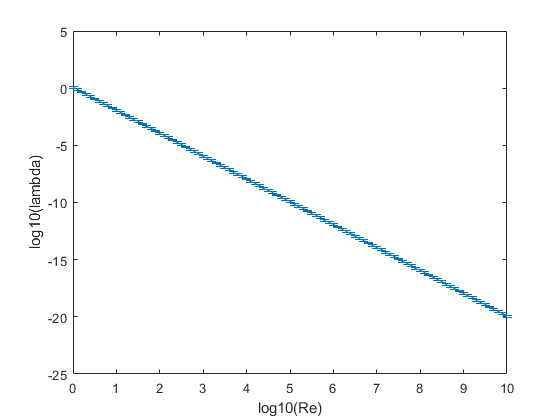
This picture is so strange... I guess it's wrong