Introduction

Good luck, eat chicken tonight ~ today, I played with my friends to eat chicken and experienced various death methods. I was also ridiculed that there are 100 death methods for girls to eat chicken, such as being swung to death by fist, parachuting to the edge of the roof, playing chicken as a flying car, being killed by car skill show, and being burned by teammates with a burning bottle. This kind of game is a game for me to understand that there is still this way of death. 

But I still have to pretend that I'm addicted to learning, so today I'll use the real data of chicken eating competition to see how to improve your probability of eating chicken.

So let's use Python and R for data analysis to answer the following soul questions?

For more complete source code and Python learning materials, click this line of font

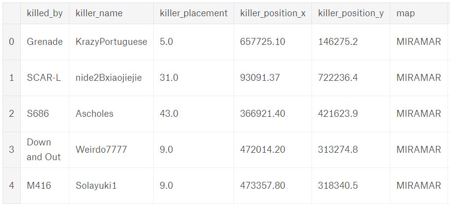
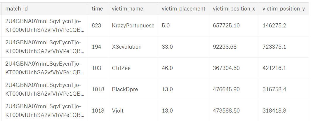
First, let's look at the following data:

1, Where is it dangerous to jump?

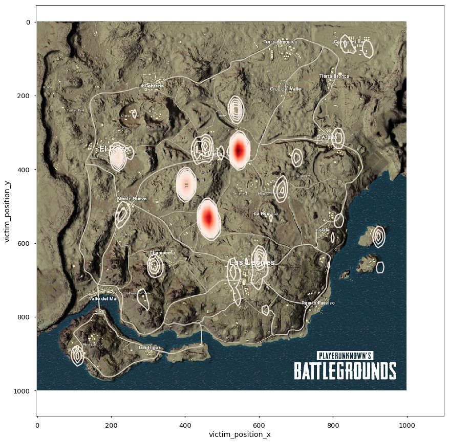
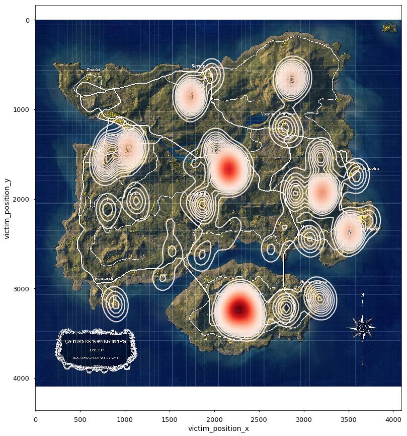
For a conscientious player like me who has always liked to live in poverty, after countless painful experiences of landing into a river, I will never choose to jump into a city with dense buildings such as P city. It's important to be poor, but it's important to keep my life. So we decided to count which places are easier to land into rivers? We screened out the locations of players who died in the first 100 seconds for visual analysis. The power station, piccado, villa area and Yibo city of passion desert map are the most dangerous, and the railway station and thermal power plant are relatively safe. P City, military base, school, hospital, nuclear power plant and air raid shelter in Jedi island are absolutely dangerous areas. The material rich port G is actually relatively safe.

import numpy as np
 2import matplotlib.pyplot as plt
 3import pandas as pd
 4import seaborn as sns
 5from scipy.misc.pilutil import imread
 6import matplotlib.cm as cm
 7
 8#Import partial data
 9deaths1 = pd.read_csv("deaths/kill_match_stats_final_0.csv")
10deaths2 = pd.read_csv("deaths/kill_match_stats_final_1.csv")
11
12deaths = pd.concat([deaths1, deaths2])
13
14#Print the first 5 columns and understand the variables
15print (deaths.head(),'\n',len(deaths))
16
17#Two kinds of maps
18miramar = deaths[deaths["map"] == "MIRAMAR"]
19erangel = deaths[deaths["map"] == "ERANGEL"]
20
21#Heat map of death 100 seconds before the start
22position_data = ["killer_position_x","killer_position_y","victim_position_x","victim_position_y"]
23for position in position_data:
24    miramar[position] = miramar[position].apply(lambda x: x*1000/800000)
25    miramar = miramar[miramar[position] != 0]
26
27    erangel[position] = erangel[position].apply(lambda x: x*4096/800000)
28    erangel = erangel[erangel[position] != 0]
29
30n = 50000
31mira_sample = miramar[miramar["time"] < 100].sample(n)
32eran_sample = erangel[erangel["time"] < 100].sample(n)
33
34# miramar thermodynamic diagram
35bg = imread("miramar.jpg")
36fig, ax = plt.subplots(1,1,figsize=(15,15))
37ax.imshow(bg)
38sns.kdeplot(mira_sample["victim_position_x"], mira_sample["victim_position_y"],n_levels=100, cmap=cm.Reds, alpha=0.9)
39
40# Ergel thermodynamic diagram
41bg = imread("erangel.jpg")
42fig, ax = plt.subplots(1,1,figsize=(15,15))
43ax.imshow(bg)
44sns.kdeplot(eran_sample["victim_position_x"], eran_sample["victim_position_y"], n_levels=100,cmap=cm.Reds, alpha=0.9)

2, Hang on or go out?

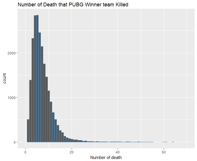
Do I stay in the room or go out to fight with the enemy? Because the scale of the competition is different, the competition data with more than 90 participants are selected, and then the team is selected_ Placement is the data of the team that successfully ate chicken in the end:

1. First, the average number of enemies killed by the chicken eating team is calculated. The competition data of the four person mode is excluded here, because the teams with too many people will become meaningless due to the wide average number;

2. Therefore, we consider counting the number of enemies killed by the members who survived to the last in each group by grouping, but it is found that the data statistics survival time variable is recorded according to the final survival time of the team, so the idea fails;

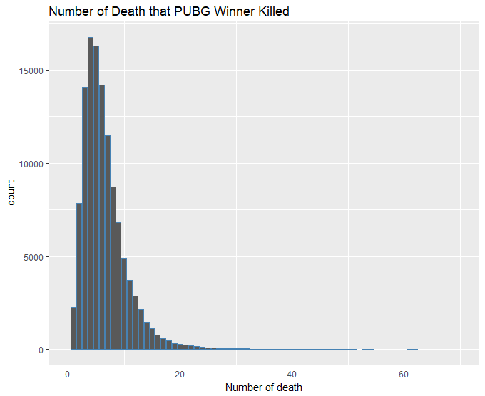
3. Finally, count the number of kills in each chicken eating team. The data of single player mode is excluded here, because the number of single player mode is the number of kills in each group. Finally, it was found that the number of kills reached 60. I doubt whether it is open. If you want to eat chicken, you still have to go out and practice shooting. You can't just go around.

library(dplyr)
 2library(tidyverse)
 3library(data.table)
 4library(ggplot2)
 5pubg_full <- fread("../agg_match_stats.csv")
 6# Average number of enemies killed by chicken eating team
 7attach(pubg_full)
 8pubg_winner <- pubg_full %>% filter(team_placement==1&party_size<4&game_size>90) 
 9detach(pubg_full)
10team_killed <- aggregate(pubg_winner$player_kills, by=list(pubg_winner$match_id,pubg_winner$team_id), FUN="mean")
11team_killed$death_num <- ceiling(team_killed$x)
12ggplot(data = team_killed) + geom_bar(mapping = aes(x = death_num, y = ..count..), color="steelblue") +
13  xlim(0,70) + labs(title = "Number of Death that PUBG Winner team Killed", x="Number of death")
14
15# Number of players killed by chicken eating team
16pubg_winner <- pubg_full %>% filter(pubg_full$team_placement==1) %>% group_by(match_id,team_id)
17attach(pubg_winner)
18team_leader <- aggregate(player_survive_time~player_kills, data = pubg_winner, FUN="max")
19detach(pubg_winner)
20
21# The largest number of enemies killed in the chicken eating team
22pubg_winner <- pubg_full %>% filter(pubg_full$team_placement==1&pubg_full$party_size>1)
23attach(pubg_winner)
24team_leader <- aggregate(player_kills, by=list(match_id,team_id), FUN="max")
25detach(pubg_winner)
26ggplot(data = team_leader) + geom_bar(mapping = aes(x = x, y = ..count..), color="steelblue") +
27  xlim(0,70) + labs(title = "Number of Death that PUBG Winner Killed", x="Number of death")
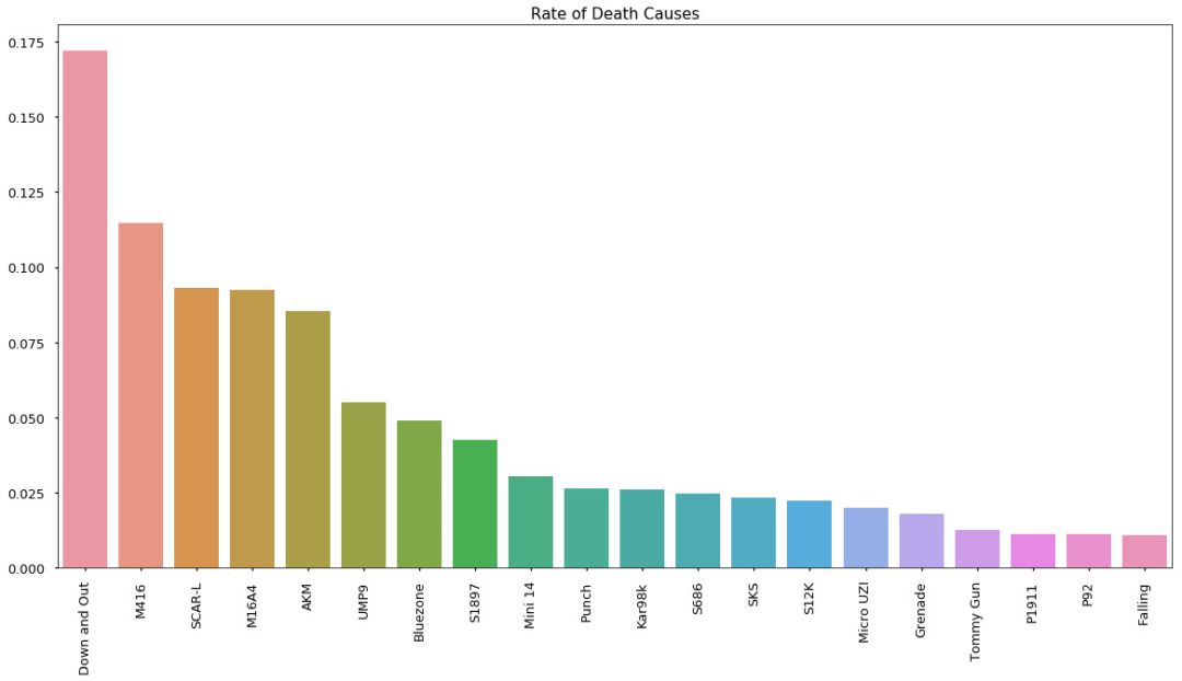
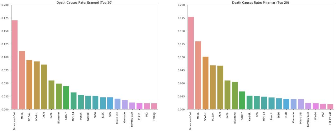
28

3, Which weapon kills more players?

When you are lucky enough to pick a good weapon, do you hesitate to choose which one? From the picture, M416 and SCAR are good weapons and relatively easy to find. It is generally recognized that Kar98k is a good gun that can kill with one shot. The reason why it ranks lower is that this gun is relatively rare in the competition, and it also needs strength to hit the enemy at once, Players like me who pick up 98k and install 8x mirror but don't cover it for 1 minute don't deserve it.

#Killer weapon ranking
 2death_causes = deaths['killed_by'].value_counts()
 3
 4sns.set_context('talk')
 5fig = plt.figure(figsize=(30, 10))
 6ax = sns.barplot(x=death_causes.index, y=[v / sum(death_causes) for v in death_causes.values])
 7ax.set_title('Rate of Death Causes')
 8ax.set_xticklabels(death_causes.index, rotation=90)
 9
10#Top 20 weapons
11rank = 20
12fig = plt.figure(figsize=(20, 10))
13ax = sns.barplot(x=death_causes[:rank].index, y=[v / sum(death_causes) for v in death_causes[:rank].values])
14ax.set_title('Rate of Death Causes')
15ax.set_xticklabels(death_causes.index, rotation=90)
16
17#The two maps are taken separately
18f, axes = plt.subplots(1, 2, figsize=(30, 10))
19axes[0].set_title('Death Causes Rate: Erangel (Top {})'.format(rank))
20axes[1].set_title('Death Causes Rate: Miramar (Top {})'.format(rank))
21
22counts_er = erangel['killed_by'].value_counts()
23counts_mr = miramar['killed_by'].value_counts()
24
25sns.barplot(x=counts_er[:rank].index, y=[v / sum(counts_er) for v in counts_er.values][:rank], ax=axes[0] )
26sns.barplot(x=counts_mr[:rank].index, y=[v / sum(counts_mr) for v in counts_mr.values][:rank], ax=axes[1] )
27axes[0].set_ylim((0, 0.20))
28axes[0].set_xticklabels(counts_er.index, rotation=90)
29axes[1].set_ylim((0, 0.20))
30axes[1].set_xticklabels(counts_mr.index, rotation=90)
31
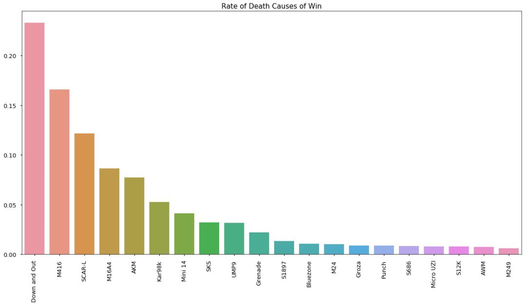
32#The relationship between eating chicken and weapons
33win = deaths[deaths["killer_placement"] == 1.0]
34win_causes = win['killed_by'].value_counts()
35
36sns.set_context('talk')
37fig = plt.figure(figsize=(20, 10))
38ax = sns.barplot(x=win_causes[:20].index, y=[v / sum(win_causes) for v in win_causes[:20].values])
39ax.set_title('Rate of Death Causes of Win')
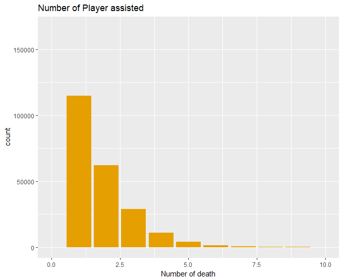
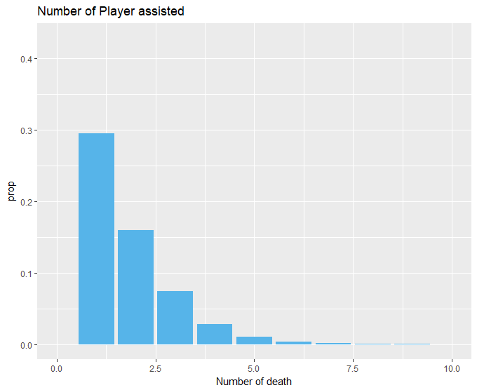
40ax.set_xticklabels(win_causes.index, rotation=90)

4, Does my teammate's assists help me eat chicken?

Sometimes I was knocked down without paying attention. Fortunately, I climbed fast and asked my teammates to save me. Here we choose the team that successfully eats chicken. The probability of the team of the member who finally receives one help eating chicken is 29%, so it's still very important for teammates to assist (don't scold my pig teammate, I can also choose not to save you.) You are also a talented person who has been saved by your teammates nine times.

library(dplyr)
 2library(tidyverse)
 3library(data.table)
 4library(ggplot2)
 5pubg_full <- fread("E:/aggregate/agg_match_stats_0.csv")
 6attach(pubg_full)
 7pubg_winner <- pubg_full %>% filter(team_placement==1) 
 8detach(pubg_full)
 9ggplot(data = pubg_winner) + geom_bar(mapping = aes(x = player_assists, y = ..count..), fill="#E69F00") +
10  xlim(0,10) + labs(title = "Number of Player assisted", x="Number of death")
11ggplot(data = pubg_winner) + geom_bar(mapping = aes(x = player_assists, y = ..prop..), fill="#56B4E9") +
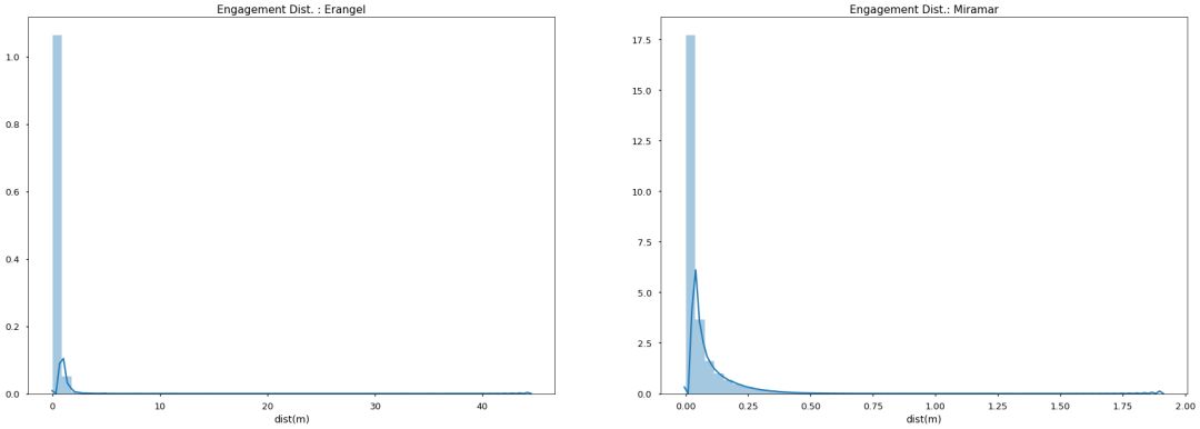
12  xlim(0,10) + labs(title = "Number of Player assisted", x="Number of death")

5, The closer the enemy is to me, the more dangerous it is?

For the killer in the data_ Position and victim_ The position variable is used to calculate the Euclidean distance. Check the linear distance between the two and the distribution of being knocked down, showing an obvious right deviation distribution. It seems that it is still necessary to observe the nearby enemy at any time, so as not to know where the enemy is when it is eliminated.

# python code: the relationship between killing and distance
 2import math
 3def get_dist(df): #distance function 
 4    dist = []
 5   for row in df.itertuples():
 6        subset = (row.killer_position_x - row.victim_position_x)**2 + (row.killer_position_y - row.victim_position_y)**2
 7        if subset > 0:
 8            dist.append(math.sqrt(subset) / 100)
 9         else:
10            dist.append(0)
11    return dist
12
13df_dist = pd.DataFrame.from_dict({'dist(m)': get_dist(erangel)})
14df_dist.index = erangel.index
15
16erangel_dist = pd.concat([erangel,df_dist], axis=1)
17
18df_dist = pd.DataFrame.from_dict({'dist(m)': get_dist(miramar)})
19df_dist.index = miramar.index
20
21miramar_dist = pd.concat([miramar,df_dist], axis=1)
22
23f, axes = plt.subplots(1, 2, figsize=(30, 10))
24plot_dist = 150
25
26axes[0].set_title('Engagement Dist. : Erangel')
27axes[1].set_title('Engagement Dist.: Miramar')
28
29plot_dist_er = erangel_dist[erangel_dist['dist(m)'] <= plot_dist]
30plot_dist_mr = miramar_dist[miramar_dist['dist(m)'] <= plot_dist]
31
32sns.distplot(plot_dist_er['dist(m)'], ax=axes[0])
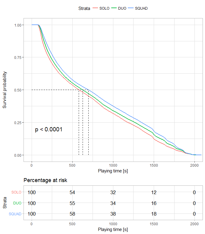
33sns.distplot(plot_dist_mr['dist(m)'], ax=axes[1])

VI. The more team members, the longer I live?

For parties in data_ Through the survival analysis of the size variable, it can be seen that under the same survival rate, the survival time of the four person team is higher than that of the two person team, and then the single person mode. Therefore, it is not unreasonable to say that many people have great strength.

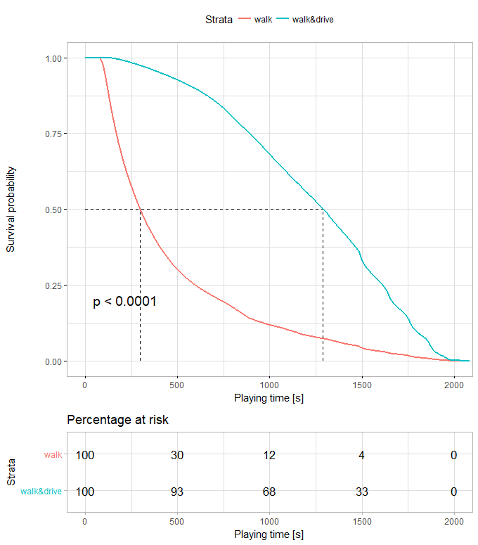
7, Do you live longer by car?

In the analysis of the cause of death, it was found that many players died in Bluezone. We naively thought that picking up the bandage could escape the poison. For the player in the data_ dist_ Through the survival analysis of ride variable, it can be seen that under the same survival rate, the survival time of players with driving experience is higher than that of players who only walk. You can't run with your legs alone.

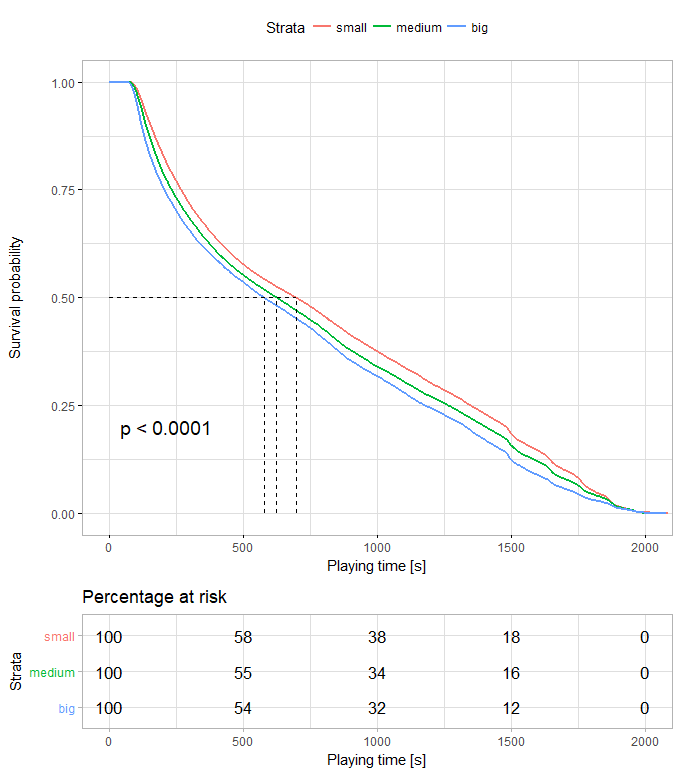
8, The more people on the island, the longer I live?

For game_ The survival analysis of size variable shows that small-scale games are easier to survive.

# R language code is as follows:
 2library(magrittr)
 3library(dplyr)
 4library(survival)
 5library(tidyverse)
 6library(data.table)
 7library(ggplot2)
 8library(survminer)
 9pubg_full <- fread("../agg_match_stats.csv")
10# Data preprocessing, classify continuous variables as classified variables
11pubg_sub <- pubg_full %>%
12  filter(player_survive_time<2100) %>%
13  mutate(drive = ifelse(player_dist_ride>0, 1, 0)) %>%
14  mutate(size = ifelse(game_size<33, 1,ifelse(game_size>=33 &game_size<66,2,3)))
15# Create a living object
16surv_object <- Surv(time = pubg_sub$player_survive_time)
17fit1 <- survfit(surv_object~party_size,data = pubg_sub)
18# Visual survival
19ggsurvplot(fit1, data = pubg_sub, pval = TRUE, xlab="Playing time [s]", surv.median.line="hv",
20           legend.labs=c("SOLO","DUO","SQUAD"), ggtheme = theme_light(),risk.table="percentage")
21fit2 <- survfit(surv_object~drive,data=pubg_sub)
22ggsurvplot(fit2, data = pubg_sub, pval = TRUE, xlab="Playing time [s]", surv.median.line="hv",
23           legend.labs=c("walk","walk&drive"), ggtheme = theme_light(),risk.table="percentage")
24fit3 <- survfit(surv_object~size,data=pubg_sub)
25ggsurvplot(fit3, data = pubg_sub, pval = TRUE, xlab="Playing time [s]", surv.median.line="hv",
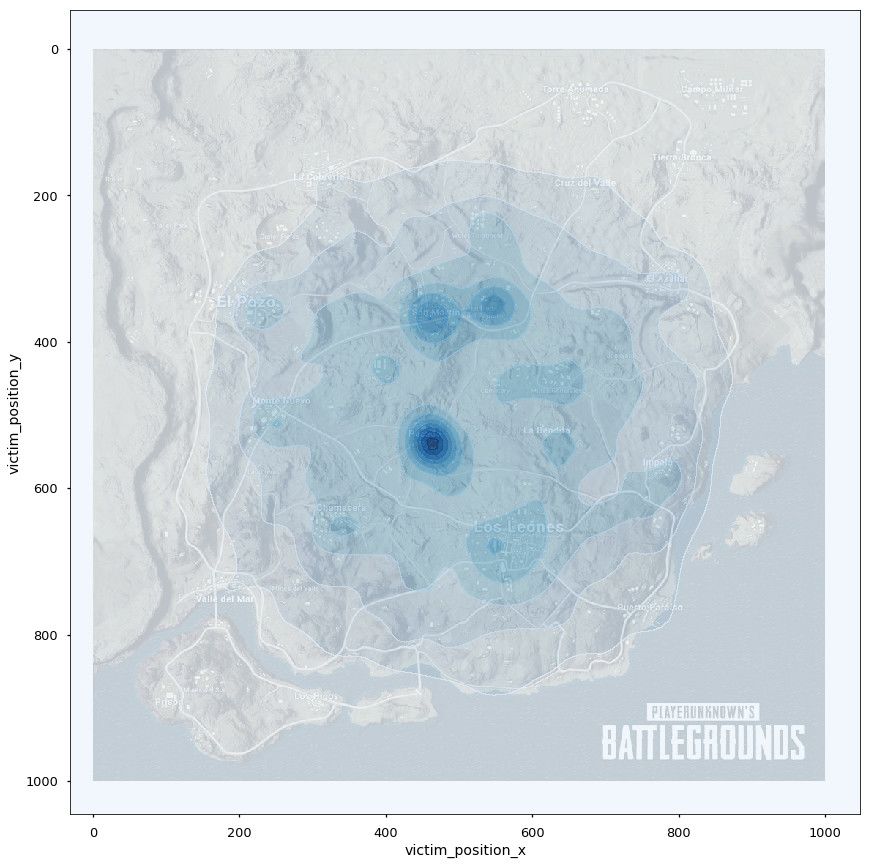
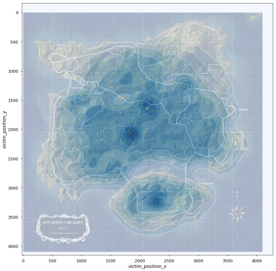
26           legend.labs=c("small","medium","big"), ggtheme = theme_light(),risk.table="percentage")

IX. where is the last poison ring likely to appear?

How to predict where the last poison circle will appear in the face of me who can survive to the end. From table agg_ match_ Find the first ranked team based on stats data, and then follow match_id grouping, find the player in the grouped data_ survive_ The maximum value of time, and then match the table kill accordingly_ match_ stats_ According to the data in final, the location of the second death is taken from these data. It is found that the poison circle in passion desert is obviously more concentrated, which probably appears in piccado, St. Martin and villa areas. Jedi islands are more random, but you can still see that military bases and mountains are more likely to be the last poison circle.

#Last poison ring position
 2import matplotlib.pyplot as plt
 3import pandas as pd
 4import seaborn as sns
 5from scipy.misc.pilutil import imread
 6import matplotlib.cm as cm
 7
 8#Import partial data
 9deaths = pd.read_csv("deaths/kill_match_stats_final_0.csv")
10#Import aggregate data
11aggregate = pd.read_csv("aggregate/agg_match_stats_0.csv")
12print(aggregate.head())
13#Find out where the last three died
14
15team_win = aggregate[aggregate["team_placement"]==1] #The first team
16#Find out the player who lives the longest in the first team of each game
17grouped = team_win.groupby('match_id').apply(lambda t: t[t.player_survive_time==t.player_survive_time.max()])
18
19deaths_solo = deaths[deaths['match_id'].isin(grouped['match_id'].values)]
20deaths_solo_er = deaths_solo[deaths_solo['map'] == 'ERANGEL']
21deaths_solo_mr = deaths_solo[deaths_solo['map'] == 'MIRAMAR']
22
23df_second_er = deaths_solo_er[(deaths_solo_er['victim_placement'] == 2)].dropna()
24df_second_mr = deaths_solo_mr[(deaths_solo_mr['victim_placement'] == 2)].dropna()
25print (df_second_er)
26
27position_data = ["killer_position_x","killer_position_y","victim_position_x","victim_position_y"]
28for position in position_data:
29    df_second_mr[position] = df_second_mr[position].apply(lambda x: x*1000/800000)
30    df_second_mr = df_second_mr[df_second_mr[position] != 0]
31
32    df_second_er[position] = df_second_er[position].apply(lambda x: x*4096/800000)
33    df_second_er = df_second_er[df_second_er[position] != 0]
34
35df_second_er=df_second_er
36# Ergel thermodynamic diagram
37sns.set_context('talk')
38bg = imread("erangel.jpg")
39fig, ax = plt.subplots(1,1,figsize=(15,15))
40ax.imshow(bg)
41sns.kdeplot(df_second_er["victim_position_x"], df_second_er["victim_position_y"], cmap=cm.Blues, alpha=0.7,shade=True)
42
43# miramar thermodynamic diagram
44bg = imread("miramar.jpg")
45fig, ax = plt.subplots(1,1,figsize=(15,15))
46ax.imshow(bg)
47sns.kdeplot(df_second_mr["victim_position_x"], df_second_mr["victim_position_y"], cmap=cm.Blues,alpha=0.8,shade=True)


Get data address:

 end

This sharing is over now ~ I hope you like it! Remember to make up a series for Xiao before you leave~

The support of my family is my biggest motivation to update! 💪🎮 Finally, I wish you all good luck ~ eat chicken tonight