Actual battle of financial risk control -- credit feature derivation and screening (top 1 of China Mobile crowd portrait competition)

Deep mining of operator variables

We take the characteristics of this competition as an example to describe:

1. Whether the user's real name system has passed the verification of whether 1 is yes and 0 is No. at present, in China, mobile phone cards are basically bound with ID cards. Of course, there are still business activities such as buying and selling so-called flow cards in some backward areas. Generally, such features are often used as anti fraud features and part of anti fraud rules. In addition, The ID card data used by the user's real name system is generally available, and the segmentation and extraction of variables for the ID card is also a common derivative means:

Firstly, 11 here represents the code of the province. We often use the code table to convert the code into specific plaintext: (some code tables are listed below)

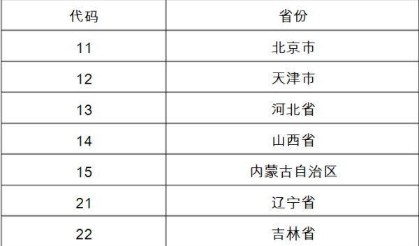
Here we can derive that the user's province is Beijing

Similarly, the 3rd and 4th digits represent the city code, the 5th and 6th digits represent the code of the district and county, the 7th to 14th digits represent the year of birth, the month, day, 15th and 16th digits represent the code of the local police station, the 17th digit represents the gender, the odd number represents the male, the even number represents the female, and the 18th digit is the check code, which is calculated by the number compilation unit according to the unified formula If the tail number is 0 to 9, there will be no X. if the tail number is 10, it will be replaced by X.

For cities, districts and counties, there is usually a corresponding code table to extract the location characteristics of users;

According to the date of birth of citizens, their age and constellation can be calculated;

The gender can be obtained by gender coding

2. According to the user's package, you can know whether the user is a college student

Now, many colleges and universities have launched preferential packages for college students, so you can judge whether the user is a college student or an office worker;

3. Blacklisted customers

Definition of operator blacklist users:

1. Users whose accounts are cancelled due to overdue arrears;

2. Malicious arrearage users (such as maliciously defrauding the telephone charges of international information stations, maliciously defrauding the telephone charges of roaming in different places, stealing calls, etc.);

3. Users suspected of SMS fraud, fraud and other criminal acts determined by the public security organ;

4. Users without owner blacklist: users who meet the above conditions without customer data, etc.

Generally, in the process of score card development, such features are mostly used to screen users as part of the anti fraud rules

4. Operators and high-risk users

It refers to four types of high-risk customers: super set, double card, double reduction and low consumption

5. User's network time

Generally, operators will also the characteristics of the length of time users spend on the Internet. This can be found by manually going to the corresponding business hall or telephone inquiry

6. User payment record

Operators generally keep the payment records of users, that is, the consumption flow information of users. There are many processing methods for this feature:

(1) . time window function, which counts the user's last consumption amount, and the sum, mean, maximum, minimum and standard deviation of the user's consumption records in the last week, month, three months, half a year, one year and three years;

(2) . time interval between the last consumption of users

(3) For the daily information of user's account balance, we will have arrears every month. The behavior patterns of different users are different. Some users like to pay more, and some users like to pay just right. Therefore, there will be some differences in each user's account balance. Then, for the sequence data of account balance, we can still use the time window function, Count the user's latest account balance, the latest week..... For three years, if the user's online time is short, the calculation result is often null, and we need to record the null value separately;

(4) . user payment, that is, some users will pay after the arrears, while others will pay before the arrears. There are differences in their behavior patterns. The user's payment behavior pattern can be described by calculating the time difference between the user's monthly payment date and the call bill date, and then the sum, mean, maximum, minimum, etc. in different time periods according to the time window Standard deviation, etc

Note: for the above sequence features, we can try to use automatic learning features such as CNN, RNN, attention and transformer to extract their potential features. For example, we can use LSTM for supervised modeling and then remove their hidden representation, or directly use the score of model output as a higher-order abstract feature automatically obtained by deep learning

7. User call record

User call record can be said to be a data type that can play out flowers. The most basic:

(1) The average, sum, standard deviation, etc. of the number of calls per week, month, March, half a year, one year, three years, etc;

(2) The average, sum, standard deviation, etc. of the user's call time every week, month, March, half a year, one year, three years, etc;

(3) . the average, sum and standard deviation of call time / number of users at home and abroad every week, month, March, half a year, one year and three years;

Many feature derivation methods can be used for the user's call records

In addition, more importantly, according to the user's call time and call situation, we can easily and intuitively construct the social map of the user's call record: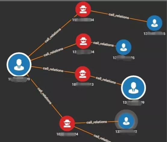
Then, combined with traditional graph algorithms, even graph embedding and GNN, try to extract features, and get the implicit social features of users to enhance the effect of downstream traditional machine learning tasks

However, it is a pity that the call records of operators have become more and more difficult to obtain

Common characteristic engineering means

1. Addition, subtraction, multiplication, division, square root, logarithm transformation, box division, etc. between continuous features;

2. Cross between category features, feature coding, box division, embedding, etc

3. Time window, applicable to the above two features, statistical features under different time windows of continuous features, counting under different time windows of categories, etc;

4. High order feature engineering is often combined with deep learning. Embedding of sequence features, embedding of id features and so on are suitable for continuous and category

Here, let's expand the processing of id features, because the processing of id features is very mature in the field of recommendation system. id features often appear in risk control, which is also a rare thing with technical content in risk control:

Basic attribute characteristics, the original characteristics of users and goods. Taking risk control as an example, user attributes include users' occupation, gender, work city, company attributes, etc. typical commodity attributes include the category of app s installed on users' mobile phones, the category of loan products borrowed by users, etc

Statistical features, common time window function (the scientific name of this thing was originally called histogram region, which can be seen in the boss's article: https://zhuanlan.zhihu.com/p/76415842 ), statistics of the user's behavior of goods in different time windows in the past, such as click / view / download / purchase; Similarly, the statistics of the above behaviors of items in different time windows also include all kinds of group by count min max mean median processing of all data;

Contextual features, such as the user's current geographical location, the transaction time, whether the day is a rest day, holiday, etc., describe the characteristics of the user's "state" when the transaction occurs;

High-order cross feature, multi-order category cross feature and gbdt cross feature are typical representatives;

Representation learning, text feature embedding, image feature embedding, sequence feature embedding, etc., all things can be embedded;

textgcn this text

Specific competition process

Data list

train_dataset.zip: training data, including 50000 lines

test_dataset.zip: test set data, including 50000 rows

Data description

The data provided this time mainly includes several aspects of user information: identity characteristics, consumption ability, contacts, location trajectory and application behavior preferences. The field description is as follows:

Field list field description

Uniqueness of user code value
Whether the user's real name system has passed the verification. 1 is yes and 0 is No
User age value
Yes for college student customer 1 and no for 0
Is blacklisted customer 1 yes 0 no
Whether 4G unhealthy customer 1 is yes, 0 is no
User network age (month)
Time (month) since the last payment by the user
Last payment amount of paying user (yuan)
Average telephone consumption cost of users in recent 6 months (yuan)
Total cost of user bill in the current month (yuan)
User's current month account balance (yuan)
Whether the paying user is currently in arrears or not. 1 is yes and 0 is No
The first level of user fee sensitivity indicates that the sensitivity level is the largest. According to the results of extreme value calculation method and leaf index weight, the sensitivity level of sensitive users is generated according to the rules: first, the sensitive users are sorted in descending order according to the middle score, the sensitivity level corresponding to the first 5% of users is level 1, and the sensitivity level corresponding to the next 15% of users is level 2; The sensitivity level of the next 15% of users is level 3; The sensitivity level of the next 25% of users is level 4; Finally, 40% of users have a sensitivity level of five.
Number of people in communication circle in current month
Whether the person who often goes shopping 1 is yes, 0 is No
Average number of shopping malls in recent three months
Have you visited Fuzhou Cangshan Wanda in the current month? 1 is yes, 0 is No
Have you been to Fuzhou Sam's club in the current month? 1 is yes, 0 is No
Whether to watch movies in the current month. 1 is yes, 0 is No
Whether to visit scenic spots in the current month. 1 is yes and 0 is No
Whether the consumption of stadiums and Gymnasiums in the current month is 1, yes, 0, No
Number of online shopping applications used in the current month
Number of logistics express applications used in the current month
Total number of financial applications used in the current month
Number of video playback applications used in the current month
Number of aircraft applications used in the current month
Number of train applications used in the current month
Number of tourism information applications used in the current month

Evaluation method

The competition evaluation index adopts MAE coefficient.

The mean absolute difference is a measure of the proximity of the model prediction results to the standard results. The calculation method is as follows:

M A E = 1 n ∑ i = 1 n ∣ p r e d i − y i ∣ M A E=\frac{1}{n} \sum_{i=1}^{n}\left|p r e d_{i}-y_{i}\right| MAE=n1∑i=1n∣predi−yi∣

Including $p r e d_{i} by Anticipate measure kind book ， For the prediction sample, Is the prediction sample, y_{i} $is a real sample. The smaller the value of MAE, the closer the predicted data is to the real data.

The final result is: $Score =\frac{1}{1+M A E}$

M S E = 1 n ∑ i = 1 n ( pred i − y i ) 2 M S E=\frac{1}{n} \sum_{i=1}^{n}\left(\text {pred}_{i}-y_{i}\right)^{2} MSE=n1∑i=1n(predi−yi)2

MSE will punish the samples with larger prediction deviation, because the data will be larger and larger after adding square.

The closer the final result is to 1, the higher the score

Comprehensive exploration

First of all, as a data competition player, we should analyze and observe the data, so that we can have a general understanding of the competition question type and data. Now let's start the overall exploration of the data.

""" Import basic library """
import numpy as np
import pandas as pd
import seaborn as sns
import matplotlib.pyplot as plt


#plt.style.use("bmh")
#plt.rc('font', family='SimHei', size=13) #Display Chinese
#pd.set_option('display.max_columns',1000)
#pd.set_option('display.width', 1000)
#pd.set_option('display.max_colwidth',1000)
plt.rcParams['font.sans-serif'] = ['Heiti TC'] # Step 1 (replace sans serif font)
plt.rcParams['axes.unicode_minus'] = False

In the data list, we know that this competition has a training set compression package and a prediction set compression package, which are decompressed in the folder and directly combined for the unified processing of subsequent data content transformation.

pd.concat combines training set and test set

""" Import data """
train_data = pd.read_csv('/Users/zhucan/Desktop/train_dataset.csv')
test_data = pd.read_csv('/Users/zhucan/Desktop/test_dataset.csv')
df_data = pd.concat([train_data, test_data], ignore_index=True)
df_data

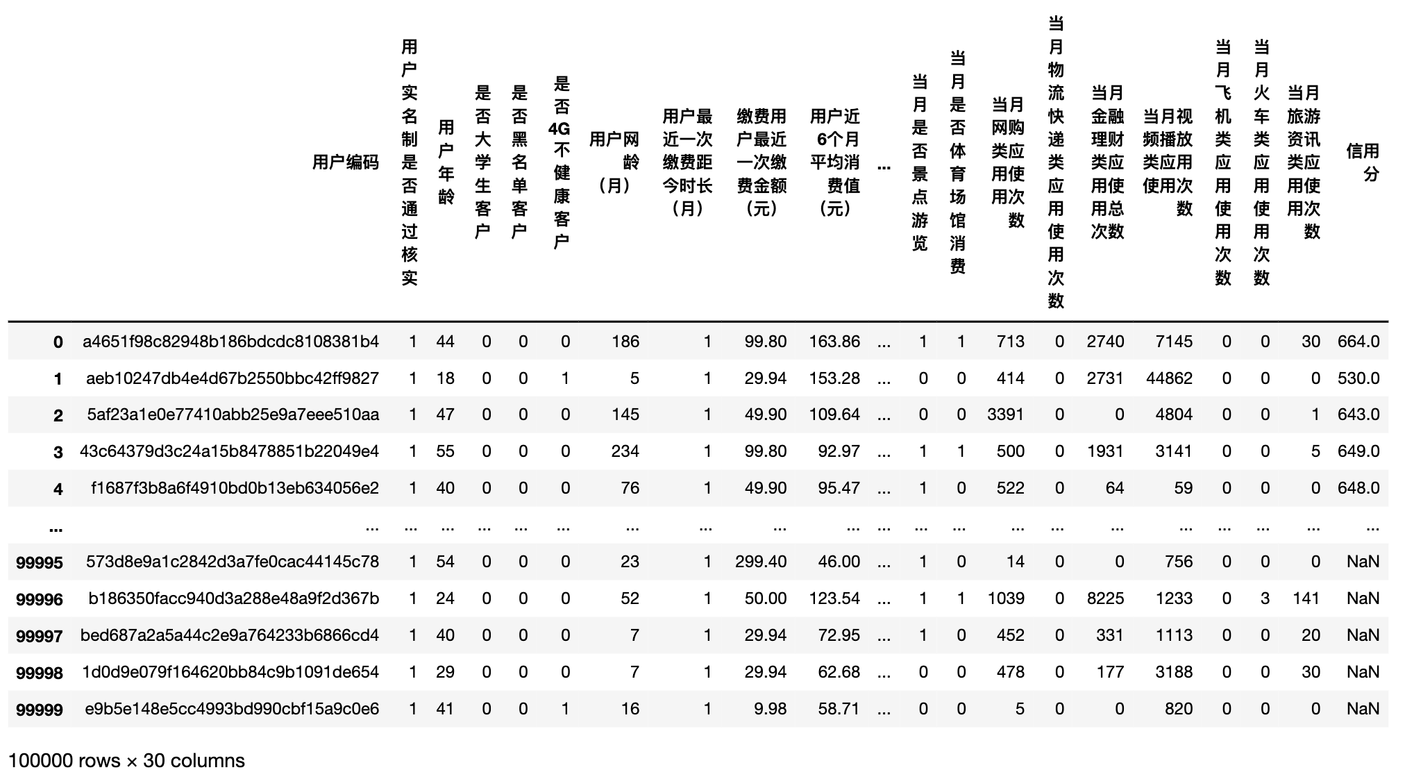
""" Data properties """
df_data.info() #It can be seen that there are no missing values
#<class 'pandas.core.frame.DataFrame'>
#Int64Index: 100000 entries, 0 to 49999
#Data columns (total 30 columns):
# #   Column           Non-Null Count   Dtype  
#---  ------           --------------   -----  
# 0 user code 100000 non null object 
# 1. Whether the user real name system has passed the verification 100000 non null Int64  
# 100000 int64-non null users  
# 3 is it a non null Int64  
# 4 is there a blacklist customer 100000 non null Int64  
# 5 is 4G unhealthy customer 100000 non null Int64  
# 6 user network age (month) 100000 non null Int64  
# 7. Time (month) since the user last paid 100000 non null Int64  
# 8 the last payment amount of the paying user (yuan) 100000 non null float64
# 9. Average consumption value of users in recent 6 months (yuan) 100000 non null float64
# 10. The total cost of the user's bill in the current month (yuan) 100000 non null float64
# 11. User's account balance in the current month (yuan) 100000 non null Int64  
# 12 whether the paying user currently owes 100000 non null Int64  
# 13. User fee sensitivity 100000 non null Int64  
# 14. The number of people in the communication circle in the current month is 100000 non null Int64  
# 15 are there 100000 non null Int64 people who often go shopping  
# 16 the average number of shopping malls in recent three months is 100000 non null Int64  
# 17. Have you visited Fuzhou Cangshan Wanda 100000 non null Int64 in that month  
# 18. Have you been to Fuzhou Sam's Club 100000 non null Int64 in the current month  
# 19. Did you watch 100000 non null Int64 movies in that month  
# 20 whether there are 100000 non null Int64 scenic spots in the current month  
# 21. Does the stadium consume 100000 non null Int64 in the current month  
# 22 number of online shopping applications used in the current month 100000 non null Int64  
# 23. The number of usage of logistics express applications in the current month is 100000 non null Int64  
# 24. The total number of financial applications used in that month was 100000 non null Int64  
# 25 video playback applications used 100000 times in the current month non null Int64  
# 26 the number of aircraft applications used in that month was 100000 non null Int64  
# 27 the number of train applications used in the current month is 100000 non null Int64  
# 28 tourism information applications used 100000 times in the current month non null Int64  
# 29 credit score 50000 non null float64
#dtypes: float64(4), int64(25), object(1)
#memory usage: 23.7+ MB
print("Common dataset:", df_data.shape[0])
print("Common test set:", test_data.shape[0])
print("Common training set:", train_data.shape[0])
#Total data set: 100000
#Total test set: 50000
#Total training set: 50000

Conclusion: the data set corresponds to the data list, indicating that there is no download error in our data. After 100000 rows are merged, it can be seen that the characteristic columns of the merged data set are all numerical characteristics and there are no missing values. Here, at the beginning of the game, the difference between a novice and a data sensitive expert begins to be reflected. Novices usually ignore this information directly. But let's try to reason that there should be a difference in the number of times that China Mobile obtains a mobile phone information store that never opens location and a home mobile phone information store that never moves. Then, never opening location is a missing value, but it does not appear in the game. After data search and investigation, it is found that in fact, the sponsor directly fills all missing values as 0, resulting in no missing values in the data set;

""" Count how many categories each feature has """
for i,name in enumerate(df_data.columns):
name_sum = df_data[name].value_counts().shape[0]
print("{},{} The number of feature categories is:{}".format(i + 1, name, name_sum))
#1. Number of user coding feature categories: 100000
# 2. Whether the user real name system has passed the verification, and the number of feature categories is: 2
# 3. The number of user age characteristic categories is: 88
# 4. Whether the number of customer characteristic categories of college students is: 2
# 5. Whether the number of blacklisted customer feature categories is: 2
# 6. Are 4G unhealthy customers? The number of characteristic categories is: 2
# 7. The number of characteristic categories of user network age (month) is 283
# 8. The number of characteristic categories of the time (month) since the user's last payment is: 2
# 9. The number of characteristic categories of the latest payment amount (yuan) of paying users is 532
# 10. The number of characteristic categories of users' average consumption value (yuan) in recent 6 months is 22520
# 11. The number of characteristic categories of the total expense (yuan) of the user bill in the current month is 16597
# 12. The number of characteristic categories of user's current month account balance (yuan) is 316
# 13. The number of characteristic categories of whether the paying user is currently in arrears is: 2
# 14. The number of user fee sensitivity feature categories is: 6
# 15. The number of characteristic categories of the number of people in the communication circle in the current month is 554
# 16. The number of characteristic categories of people who often visit shopping malls is: 2
# 17. The average number of shopping malls in recent three months and the number of characteristic categories are: 93
# 18. Have you visited Fuzhou Cangshan Wanda in that month? The number of characteristic categories is: 2
# 19. Have you been to Fuzhou Sam's club in the current month? The number of characteristic categories is: 2
# 20. The number of feature categories of whether to watch movies in the current month is: 2
# 21. Whether there are scenic spots in the current month? The number of tourist feature categories is: 2
# 22. Whether the consumption characteristics of stadiums and Gymnasiums in the current month are: 2
# 23. The usage times of online shopping applications in the current month and the number of characteristic categories are: 8382
# 24. The number of usage times of logistics express applications in the current month is 239
# 25. The total number of financial management applications used in the current month and the number of characteristic categories are: 7232
# 26. The number of video playback applications used in the current month is 16067
# 27. The number of characteristic categories of aircraft applications in the current month is 209
# 28. The number of characteristic categories of the number of train applications used in the current month is 180
# 29. The number of characteristic categories of usage times of tourism information applications in the current month is 934
# 30. The number of credit characteristic categories is 278

""" data statistics """
df_data.describe()

df_data['Credit score'].isnull()
#0        False
#1        False
#2        False
#3        False
#4        False
#         ...  
#99995     True
#99996     True
#99997     True
#99998     True
#99999     True
#Name: credit score, Length: 100000, dtype: bool
""" Observation training/Same distribution of test set data """
df_data[df_data['Credit score'].isnull()].describe()

df_data[df_data['Credit score'].notnull()].describe()

Primary feature exploration (data preprocessing)

Next, start to analyze the correlation between characteristics and credit score, and carry out relevant primary feature exploration. Many novices often have no way to start in feature exploration. It is recommended to explore features in the order of continuous, discrete and unstructured features

Continuous + continuous

Category + category is more complex, join and convert to text

Continuous + category similar feature coding

Unstructured

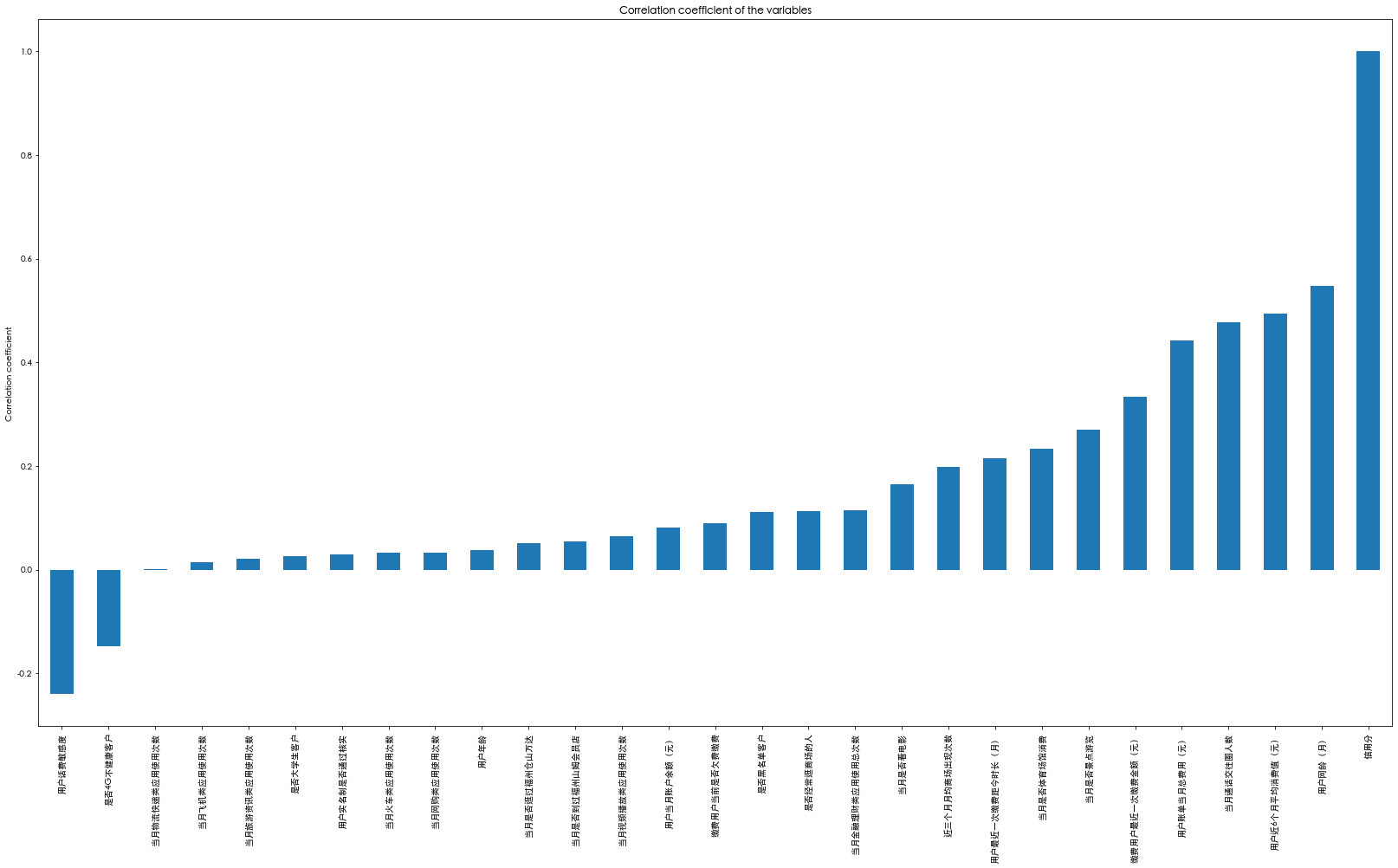
Calculate the feature correlation of each feature and label

# np.corrcoef(df_data ['whether to watch movies in the current month']. values,df_data. Credit score. values)
df_train=df_data[df_data['Credit score'].notnull()]
df_train.head()

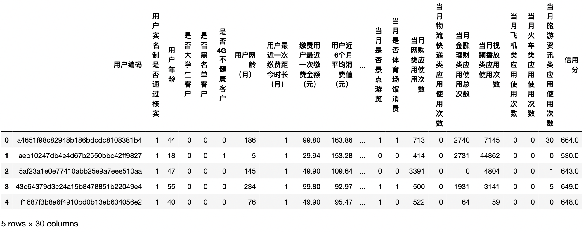
np.corrcoef(df_train['Do you watch movies that month'].values,df_train['Credit score'].values)[0,1]
#0.1653765230842276
df_train.columns
#Index(['user code', 'whether the user's real name system has been verified', 'user age', 'whether it is a college student customer', 'whether it is a blacklist customer', 'whether it is a 4G unhealthy customer', 'user's network age (month),' the length of time (month) since the last payment by the user ',' the last payment amount of the fee payer (yuan), 'the average consumption value of the user in recent 6 months (yuan),' the total cost of the user's bill in the current month (yuan), 'user's account balance in the current month (yuan),' whether the paying user is currently in arrears', 'user's phone bill sensitivity', 'number of people in the communication circle in the current month', 'whether they often visit the mall', 'average number of shopping malls in recent three months',' whether they have visited Fuzhou Cangshan Wanda in the current month ',' whether they have visited Fuzhou Sam's club in the current month ',' whether they have watched movies in the current month ', 'whether to visit scenic spots in the current month', 'whether to consume stadiums and Gymnasiums in the current month', 'number of online shopping applications in the current month', 'number of logistics express applications in the current month', 'total number of financial applications in the current month', 'number of video playback applications in the current month', 'number of aircraft applications in the current month', 'number of train applications in the current month', 'number of tourism information applications in the current month', 'credit score'] (dtype='object ')

from matplotlib.font_manager import FontProperties
myfont=FontProperties(fname='SimHei.ttf',size=14)
plt.figure(figsize=(28,15))
ax = df_train.corr()['Credit score'].sort_values().plot(kind="bar")
ax.set_title('Correlation coefficient of the variables')
ax.set_ylabel('Correlation coefficient')

x_cols=[col for col in df_train.columns if col not in ['Credit score'] if df_train[col].dtype!='object']

labels=[]
values=[]
for col in x_cols:
    labels.append(col)
    values.append(np.corrcoef(df_train[col].values,df_train['Credit score'].values)[0,1])
    
corr_df=pd.DataFrame({'col_labels':labels,'corr_values':values})
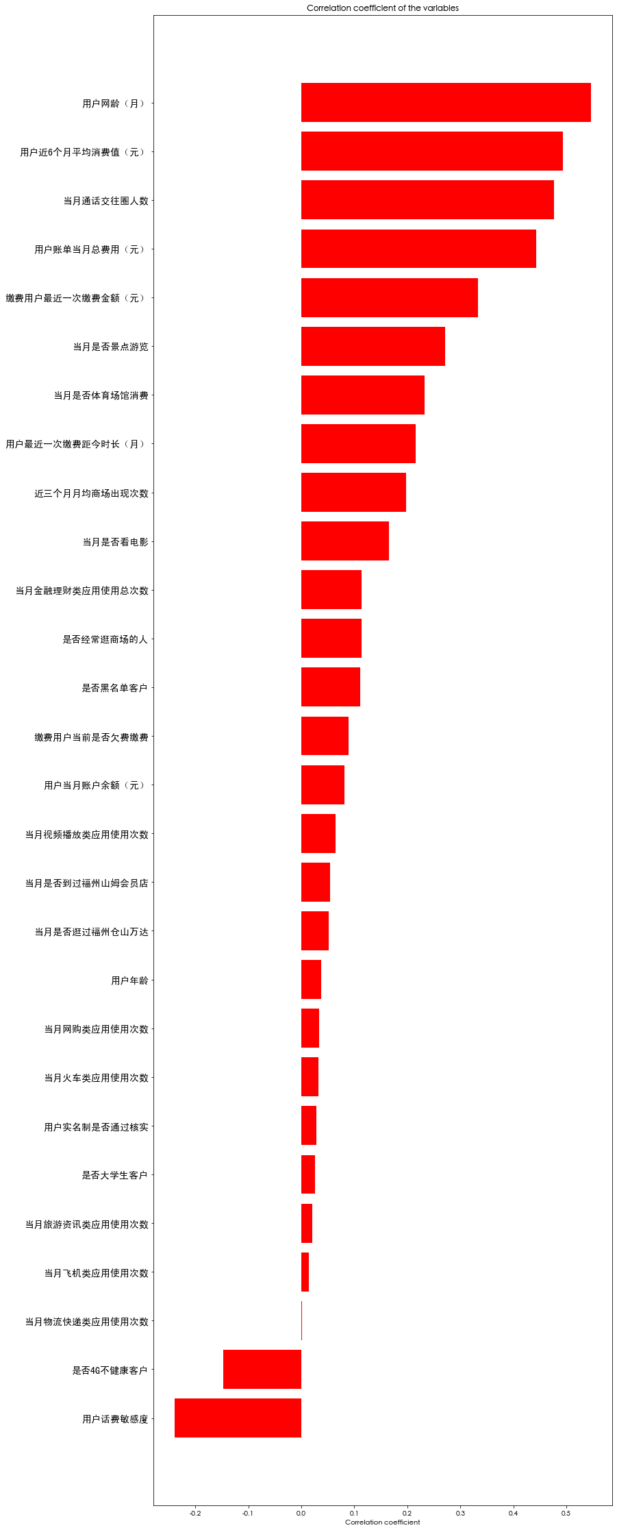
corr_df=corr_df.sort_values(by='corr_values')

fig,ax=plt.subplots(figsize=(12,40))
ind=np.arange(len(labels))
ax.barh(ind,corr_df.corr_values.values,color='r')
ax.set_yticks(ind)
ax.set_yticklabels(corr_df.col_labels.values,rotation='horizontal',fontproperties=myfont)
ax.set_xlabel('Correlation coefficient')
ax.set_title('Correlation coefficient of the variables')

# Continuous value feature
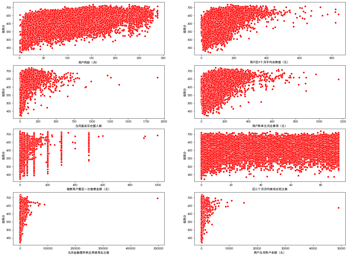
name_list=['User network age (month)','Average consumption value of users in recent 6 months (yuan)','Number of communication circles in the current month','Total cost of user bill in the current month (yuan)',
           'Last payment amount of payer (yuan)','Average number of shopping malls in recent three months','Total usage times of financial management applications in the current month','User's current month account balance (yuan)']
f, ax = plt.subplots(4, 2, figsize=(20, 15))
for i,name in enumerate(name_list):
    sns.scatterplot(data=df_train, x=name, y='Credit score', color='r', ax=ax[i // 2][i % 2])
plt.show()

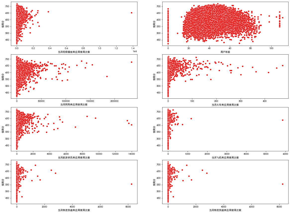
name_list=['Application video playback times in the current month','User age','Usage times of online shopping applications in the current month','Number of train applications used in the current month',
           'Usage times of tourism information applications in the current month','Number of aircraft applications used in the current month','Usage times of logistics express applications in the current month','Usage times of logistics express applications in the current month']
f, ax = plt.subplots(4, 2, figsize=(20, 15))
for i,name in enumerate(name_list):
    sns.scatterplot(data=df_train, x=name, y='Credit score', color='r', ax=ax[i // 2][i % 2])
plt.show()

# Discrete value feature
name_list = ['Whether to visit scenic spots in the current month','Whether the consumption of stadiums and Gymnasiums in the current month','Time since the user last paid (month)', 'Do you watch movies that month',
             'Do you often go shopping','Blacklisted customers','Is the paying user in arrears','Have you ever been to Fuzhou Sam's club in that month',
             'Have you visited Fuzhou Cangshan Wanda in that month', 'Whether the user's real name system has been verified','Is it a college student customer','Whether 4 G Unhealthy customers']

f, ax = plt.subplots(4, 3, figsize=(20, 15))

for i,name in enumerate(name_list):
    sns.boxplot(data=df_data, x=name, y='Credit score',ax=ax[i // 3][i % 3])
plt.show()

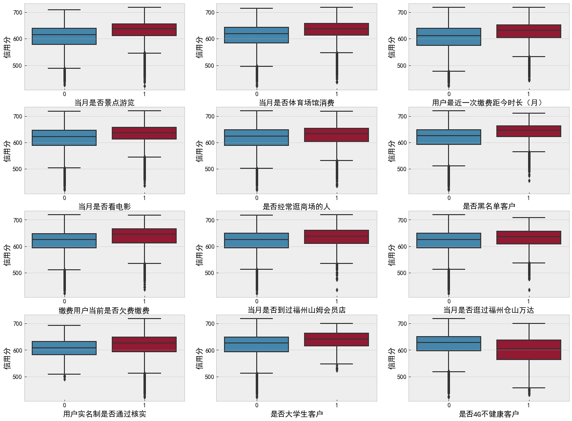
# Discrete value feature
f, ax = plt.subplots( figsize=(20, 6))
sns.boxplot(data=df_train, x='User fee sensitivity', y='Credit score', color='r')
plt.show()

Do basic processing for the data and observe the univariate correlation again

df_train.describe()

def base_process():
    transform_value_feature=['User age','User network age (month)','Number of communication circles in the current month',
                             'Average number of shopping malls in recent three months','Usage times of online shopping applications in the current month','Usage times of logistics express applications in the current month',
                             'Total usage times of financial management applications in the current month','Application video playback times in the current month', 'Number of aircraft applications used in the current month',
                             'Number of train applications used in the current month','Usage times of tourism information applications in the current month']
    
    user_fea=['Last payment amount of payer (yuan)','Average consumption value of users in recent 6 months (yuan)','Total cost of user bill in the current month (yuan)','User's current month account balance (yuan)']
    
    log_features=['Usage times of online shopping applications in the current month','Total usage times of financial management applications in the current month','Application video playback times in the current month']
    
    #Deal with outliers Here, we directly assign the value corresponding to 99.9% to the data greater than 99.9%, and assign the value corresponding to 0.1% to the data less than 0.1%
    for col in transform_value_feature+user_fea+log_features:
        ulimit=np.percentile(df_train[col].values, 99.9) #Calculate any percentage quantile of a multidimensional array
        llimit=np.percentile(df_train[col].values, 0.1)
        df_train.loc[df_train[col]>ulimit,col]=ulimit  # Direct assignment greater than 99.9%
        df_train.loc[df_train[col]<llimit,col]=llimit
        
            
    for col in user_fea+log_features:
        df_train[col]=df_train[col].map(lambda x: np.log1p(x)) #Take logarithmic change
        
    return df_train

train_df=base_process()
train_df.head()

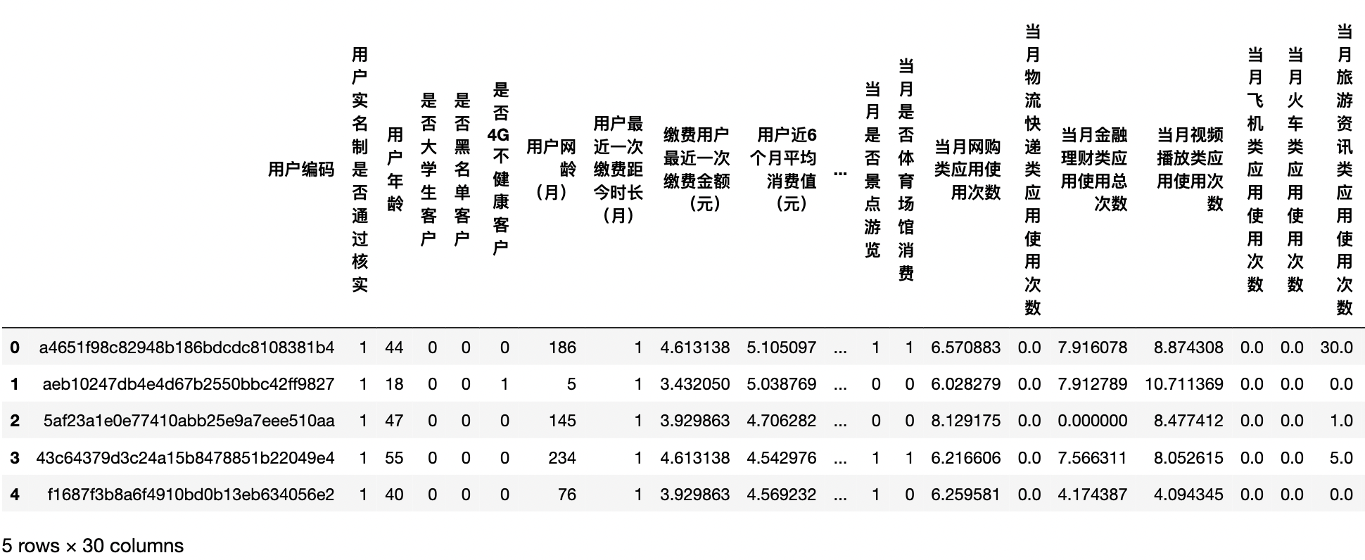
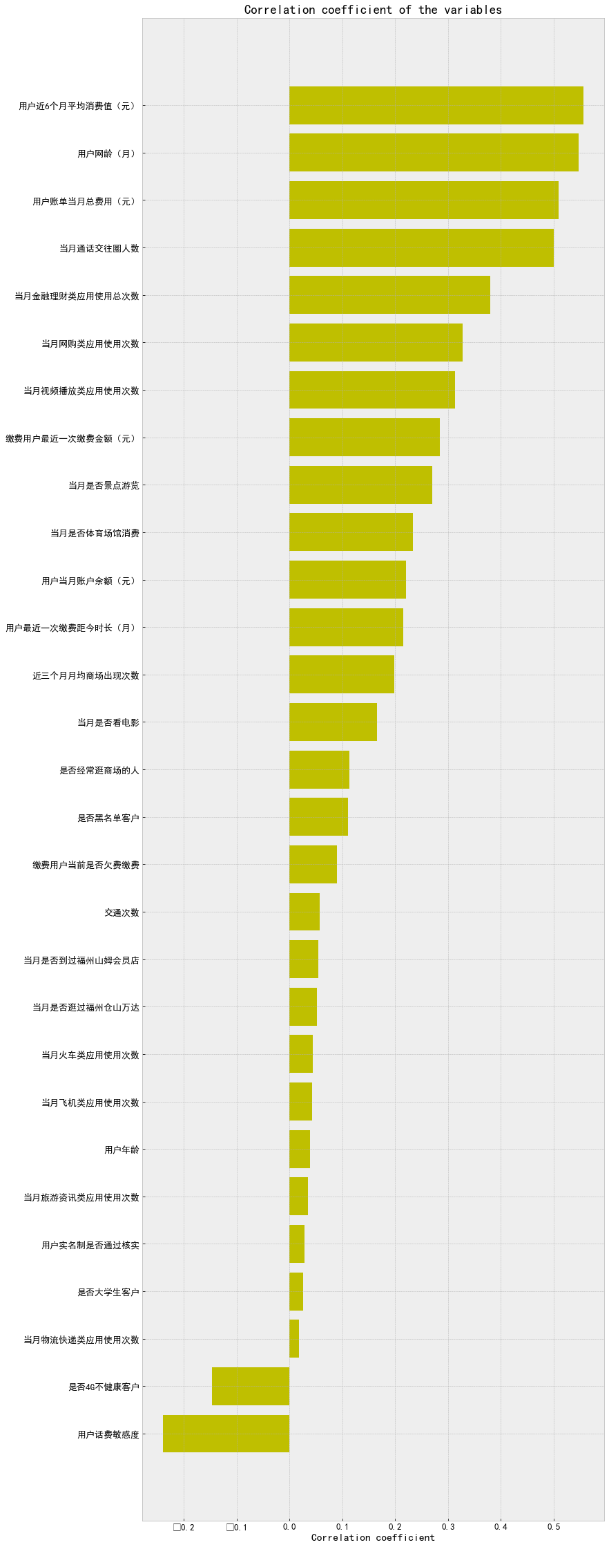
After data processing, the correlation degree is measured again

train_df['Traffic frequency']=train_df['Number of aircraft applications used in the current month']+train_df['Number of train applications used in the current month']

x_cols=[col for col in train_df.columns if col not in ['Credit score'] if train_df[col].dtype!='object']

labels=[]
values=[]
for col in x_cols:
    labels.append(col)
    values.append(np.corrcoef(train_df[col].values,train_df.Credit score.values)[0,1])
corr_df=pd.DataFrame({'col_labels':labels,'corr_values':values})
corr_df=corr_df.sort_values(by='corr_values')

ind=np.arange(len(labels))
width=0.5
fig,ax=plt.subplots(figsize=(12,40))
rects=ax.barh(ind,corr_df.corr_values.values,color='y')
ax.set_yticks(ind)
ax.set_yticklabels(corr_df.col_labels.values,rotation='horizontal')
ax.set_xlabel('Correlation coefficient')
ax.set_title('Correlation coefficient of the variables')

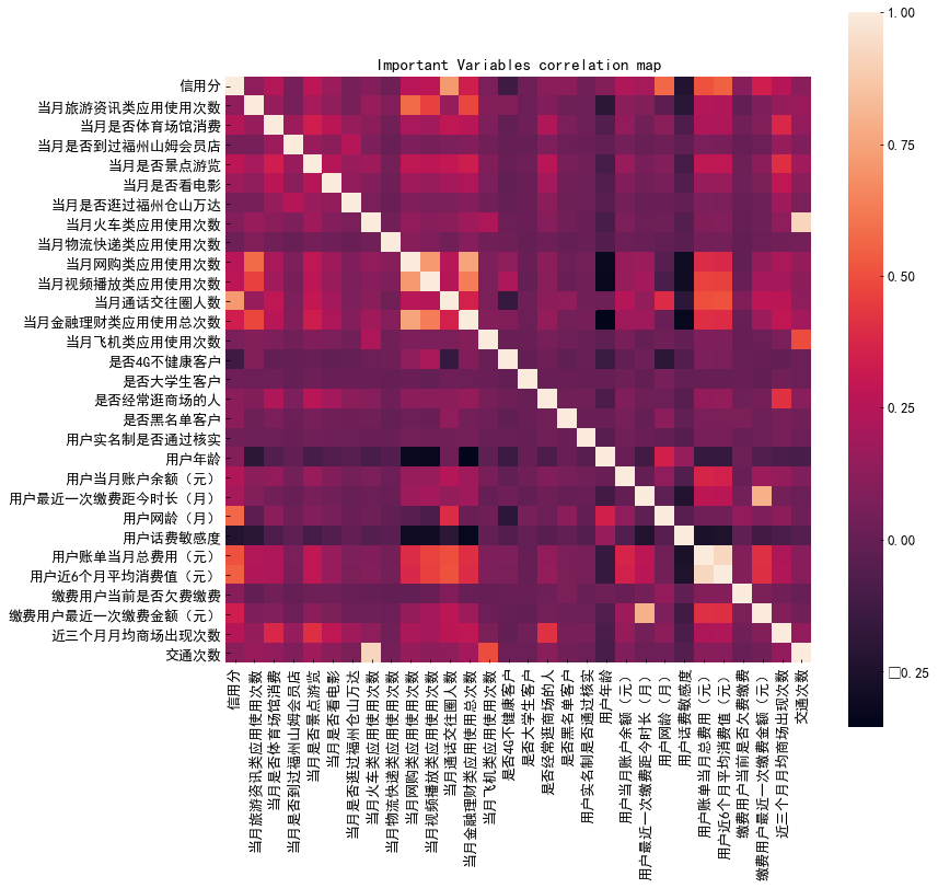
Pairwise correlation between all continuous variables

corrmat=train_df.corr(method='spearman')

f,ax=plt.subplots(figsize=(12,12))
sns.heatmap(corrmat,vmax=1,square=True)
plt.title('Important Variables correlation map',fontsize=15)

Characteristic Engineering

def get_features():
    
    df_data.loc[df_data['User age']==0,'User age']=df_data['User age'].mode() #The mode is better than the average
    
    #According to the importance of previous features, several strongly related features are processed
    df_data['Can the payment amount cover the bill of the current month']=df_data['Last payment amount of payer (yuan)']-df_data['Total cost of user bill in the current month (yuan)']
    df_data['Did the last payment exceed the average consumption']=df_data['Last payment amount of payer (yuan)']-df_data['Average consumption value of users in recent 6 months (yuan)']
    df_data['Does the bill of the current month exceed the average consumption']=df_data['Total cost of user bill in the current month (yuan)']-df_data['Average consumption value of users in recent 6 months (yuan)']
    
        
    #These features have little correlation
    df_data['Have you ever been to a high-end shopping mall']=df_data['Have you visited Fuzhou Cangshan Wanda in that month']+df_data['Have you ever been to Fuzhou Sam's club in that month']
    df_data['Have you ever been to a high-end shopping mall']=df_data['Have you ever been to a high-end shopping mall'].map(lambda x:1 if x>=1 else 0)
    df_data['whether_market_film']=df_data['Have you ever been to a high-end shopping mall']*df_data['Do you watch movies that month'] #Multiplication is used here
    df_data['whether_market_Travel']=df_data['Have you ever been to a high-end shopping mall']*df_data['Whether to visit scenic spots in the current month']
    df_data['whether_market_Gymnasium']=df_data['Have you ever been to a high-end shopping mall']*df_data['Whether the consumption of stadiums and Gymnasiums in the current month']
    df_data['whether_film_Gymnasium']=df_data['Do you watch movies that month']*df_data['Whether the consumption of stadiums and Gymnasiums in the current month']
    df_data['whether_film_Travel']=df_data['Do you watch movies that month']*df_data['Whether to visit scenic spots in the current month']
    df_data['whether_Travel_Gymnasium']=df_data['Whether to visit scenic spots in the current month']*df_data['Whether the consumption of stadiums and Gymnasiums in the current month']
    
     
    df_data['whether_market_Travel_Gymnasium']=df_data['Have you ever been to a high-end shopping mall']*df_data['Whether to visit scenic spots in the current month']*df_data['Whether the consumption of stadiums and Gymnasiums in the current month']
    df_data['whether_market_film_Gymnasium']=df_data['Have you ever been to a high-end shopping mall']*df_data['Do you watch movies that month']*df_data['Whether the consumption of stadiums and Gymnasiums in the current month']
    df_data['whether_market_film_Travel']=df_data['Have you ever been to a high-end shopping mall']*df_data['Do you watch movies that month']*df_data['Whether to visit scenic spots in the current month']
    df_data['whether_Gymnasium_film_Travel']=df_data['Whether the consumption of stadiums and Gymnasiums in the current month']*df_data['Do you watch movies that month']*df_data['Whether to visit scenic spots in the current month']
    
    df_data['whether_market_Gymnasium_film_Travel']=df_data['Have you ever been to a high-end shopping mall']*df_data['Whether the consumption of stadiums and Gymnasiums in the current month']*df_data['Do you watch movies that month']*df_data['Whether to visit scenic spots in the current month']
       
    #The data is discretized. In most cases, the data is 0 or 1, so discretization is adopted
    discretize_features=['Usage times of traffic applications','Usage times of logistics express applications in the current month','Number of aircraft applications used in the current month','Number of train applications used in the current month','Usage times of tourism information applications in the current month']
    df_data['Usage times of traffic applications']=df_data['Number of aircraft applications used in the current month']+df_data['Number of train applications used in the current month']
    
    def map_discreteze(x):
        if x==0:
            return 0
        elif x<=5:
            return 1
        elif x<=15:
            return 2
        elif x<=50:
            return 3
        elif x<=100:
            return 4
        else:
            return 5
        
    for col in discretize_features:
        
        df_data[col]=df_data[col].map(lambda x: map_discreteze(x))
            
    return df_data
           
all_data=get_features()
all_data

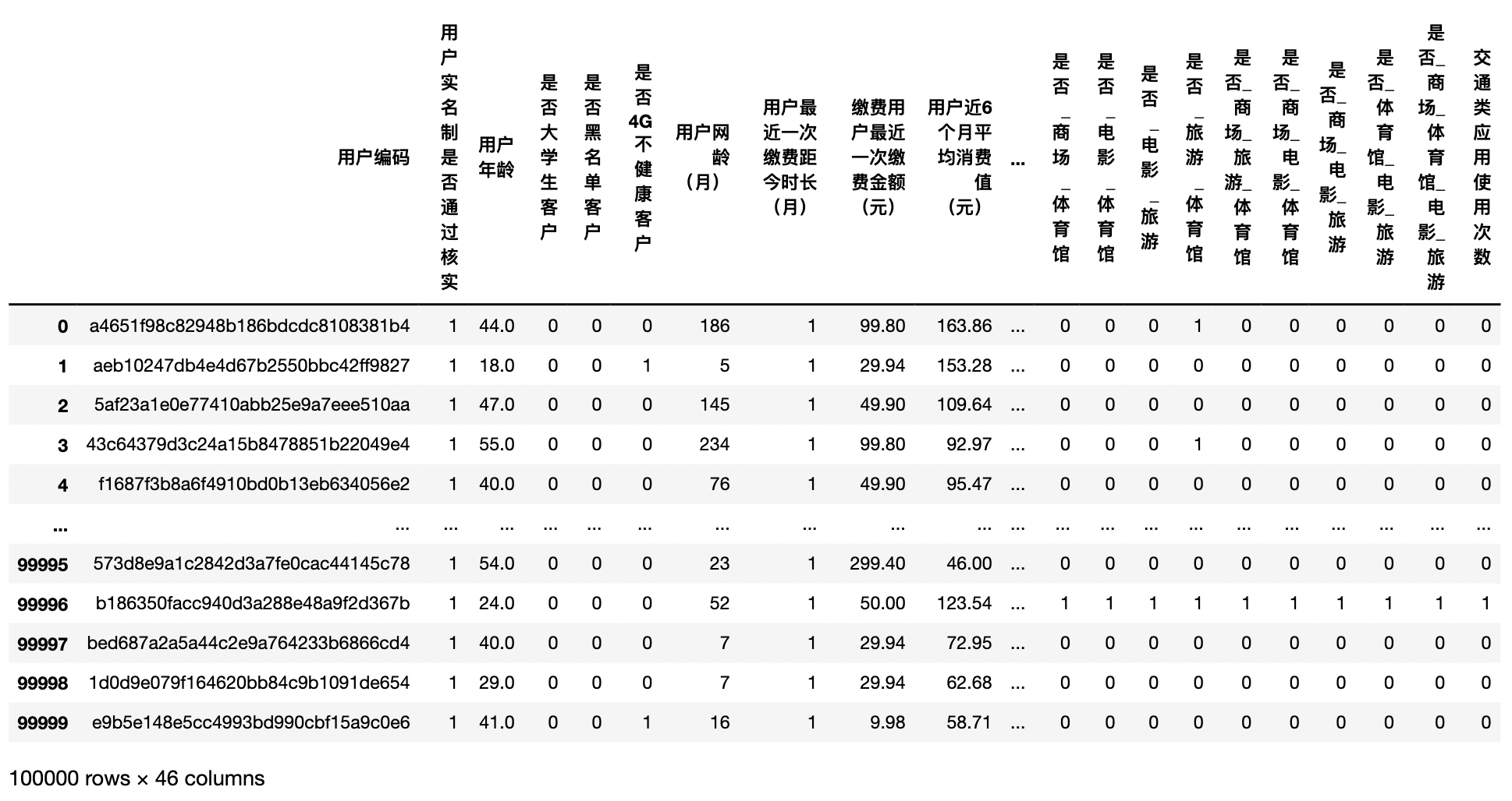
def base_process():
    transform_value_feature=['User age','User network age (month)','Number of communication circles in the current month','Did the last payment exceed the average consumption',
                             'Average number of shopping malls in recent three months','Usage times of online shopping applications in the current month','Usage times of logistics express applications in the current month','Does the bill of the current month exceed the average consumption',
                     'Total usage times of financial management applications in the current month','Application video playback times in the current month', 'Number of aircraft applications used in the current month','Number of train applications used in the current month',
                             'Usage times of tourism information applications in the current month']
    
    user_bill_features=['Last payment amount of payer (yuan)','Average consumption value of users in recent 6 months (yuan)','Total cost of user bill in the current month (yuan)','User's current month account balance (yuan)']
    
    log_features=['Usage times of online shopping applications in the current month','Total usage times of financial management applications in the current month','Application video playback times in the current month']
    
    #Handling outliers
    for col in transform_value_feature+user_bill_features+log_features:
        ulimit=np.percentile(all_data[col].values, 99.9) #Calculate any percentage quantile of a multidimensional array
        llimit=np.percentile(all_data[col].values, 0.1)
        all_data.loc[all_data[col]>ulimit,col]=ulimit  # Direct assignment greater than 99.9%
        all_data.loc[all_data[col]<llimit,col]=llimit
        
      
    for col in user_bill_features+log_features:
        all_data[col]=all_data[col].map(lambda x: np.log1p(x)) #Take logarithmic change
        
    
    train=all_data[:50000]
    test=all_data[50000:]
    return train,test   

train,test=base_process()

#Final training set and test set
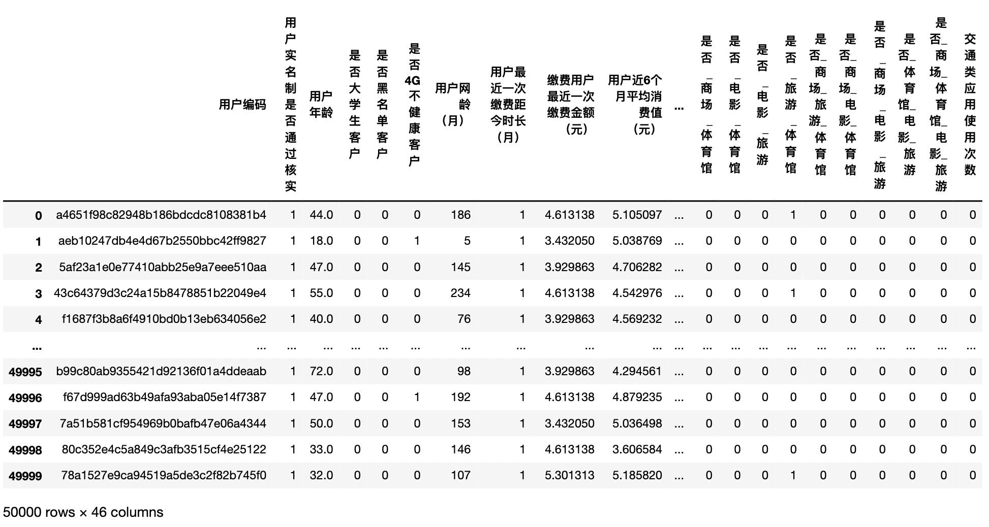
train.head()

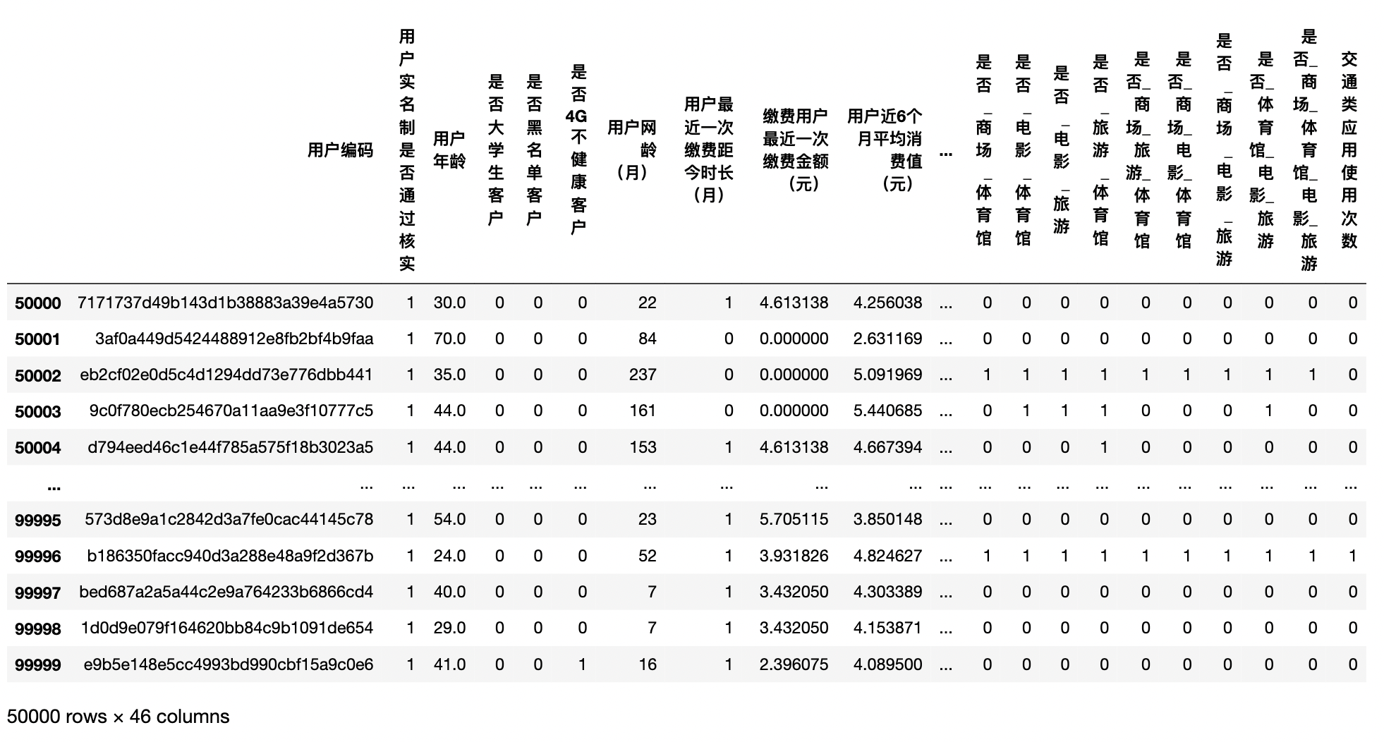
test.head()

feature_name=[col for col in train.columns if col not in ['Credit score'] if col not in ['User code'] ]
label_name=['Credit score']
train_feature=train[feature_name]
train_label=train[label_name]
test_feature=test[feature_name]

Model and parameters

from sklearn.model_selection import KFold,StratifiedKFold
from sklearn.metrics import accuracy_score
import lightgbm as lgb

def labcv_predict(train_feature,train_label):
   
    lgb_params1={
                'boosting_type':'gbdt','num_leaves':31,'reg_alpha':2.2,'reg_lambda':1.5,
                'max_depth':1,'n_estimators':2000,
                'subsample':0.8,'colsample_bytree':0.7,'subsample_freq':1,
                'learning_rate':0.03,'random_state':2019,'n_jobs':-1}
    
    clf2=lgb.LGBMRegressor(
                boosting_type='gbdt',num_leaves=31,reg_alpha=1.2,reg_lambda=1.8,
                max_depth=-1,n_estimators=2000,
                subsample=0.8,colsample_bytree=0.7,subsample_freq=1,
                learning_rate=0.03,random_state=2018,n_jobs=-1)

    
    kf=KFold(n_splits=10,random_state=2019,shuffle=True)  #Ten fold cross validation
    modell=[]
    model2=[]
    best_score=[]
    sub_list=[]
    
    t_feature=train_feature.values
    t_label=train['Credit score'].values
   

    for i,(train_index,val_index) in enumerate(kf.split(t_feature)):
        X_train=t_feature[train_index,:]
        y_train=t_label[train_index]
        X_val=t_feature[val_index,:]
        y_val=t_label[val_index]
   
        
        #First parameter prediction
        clf=lgb.LGBMRegressor(**lgb_params1)
        clf.fit(X_train,y_train,eval_set=[(X_train,y_train),(X_val,y_val)],eval_metric='mae',early_stopping_rounds=100,verbose=200)
        pred_val1=clf.predict(X_val,num_iteration=clf.best_iteration_) #Label of the predicted divided test set
        #vali_mae1=mean_absolute_error(y_val,np.round(pred_val1))
        vali_mae1=accuracy_score(y_val,np.round(pred_val1))
        #pred_test1=clf.predcit(test[feature_name],num_iteration=clf.best_iteration_) #Label of the predicted unlabeled test set
        modell.append(clf)
        
    
        
        # Second parameter prediction
        clf2.fit(X_train,y_train,eval_set=[(X_train,y_train),(X_val,y_val)],eval_metric='rmse',early_stopping_rounds=100,verbose=200)
        pred_val2=clf.predict(X_val,num_iteration=clf2.best_iteration_) #Label of the predicted divided test set
        #vali_mae2=mean_absolute_error(y_val,np.round(pred_val2))
        vali_mae2=accuracy_score(y_val,np.round(pred_val2))
        #pred_test2=clf.predcit(test_featur,num_iteration=clf2.best_iteration_) #Label of the predicted unlabeled test set
        model2.append(clf2)
        
        
        pred_val=np.round(pred_val1*0.5+pred_val2*0.5)  #The predicted label set after fusion
        vali_mae=accuracy_score(y_val,pred_val)
        best_score.append(1/(1+vali_mae))
        
        #pred_test=np.round(pred_test1*0.5+pred_test2*0.5) #Label of unlabeled test set predicted after fusion
        
        #Show feature importance
        predictors=[i for i in train_feature.columns]
        feat_imp=pd.Series(clf.feature_importances_,predictors).sort_values(ascending=False)

        #sub_list.append(pred_test)
        
        
    #pred_test=np.mean(np.array(sub_list),axis=0)
    print(best_score,'\n',np.mean(best_score),np.std(best_score))
    print('Feature importance',feat_imp)
    return pred_val,modell,model2
    
pred_result,modell,model2=labcv_predict(train_feature,train_label)
#[0.9769441187964047, 0.9798157946306095, 0.9807767752059631, 0.9805844283192783, 0.9769441187964047, 0.9815469179426777, 0.9782821365681863, 0.9788566953797964, 0.9811616954474096, 0.9775171065493647] 
#0.9792429787636096 0.0016760169355545553
#Feature importance user age 354
#Number of people in communication circle in the current month 316
#Average consumption value of users in recent 6 months (yuan) 294
#User network age (month) 252
#Whether the bill of the current month exceeds the average consumption 146
#Total cost of user bill in the current month (yuan) 111
#Number of video playback applications used in the current month 92
#User fee sensitivity 75
#The total number of financial applications used in that month was 55
#Last payment amount of payer (yuan): 54
#Usage times of tourism information applications in the current month 44
#Average number of shopping malls in recent three months 42
#Whether the payment amount can cover the bill of the current month 41
#User's current month account balance (yuan) 37
#Are 4G unhealthy customers 24
#Whether the paying user is currently in arrears 19
#Usage times of traffic applications 18
#Whether to visit scenic spots in the current month
#Usage times of online shopping applications in the current month 8
#Did the last payment exceed the average consumption by 6
#Time since the last payment by the user (month) 1
#Usage times of logistics express applications in the current month 1
#Have you been to Fuzhou Sam's Club 0 in the current month
#Whether to watch movies in the current month 0
#The number of aircraft applications used in the current month is 0
#Number of train applications used in the current month 0
#Whether the consumption of stadiums and Gymnasiums in the current month is 0
#Whether_ Gymnasium_ Film_ Travel 0
#Whether_ Shopping malls_ Film_ Travel 0
#Whether_ Shopping malls_ Film_ Gymnasium 0
#Have you visited Fuzhou Cangshan Wanda 0 in that month
#Whether_ Shopping malls_ Movie 0
#College student customer 0
#Are people who often go shopping 0
#Have you been to high-end shopping malls 0
#Whether the user's real name system has passed the verification 0
#Whether_ Shopping malls_ Travel_ Gymnasium 0
#Whether_ Shopping malls_ Gymnasium_ Film_ Travel 0
#Whether_ Travel_ Gymnasium 0
#Whether_ Film_ 0 travel
#Whether_ Film_ Gymnasium 0
#Whether_ Shopping malls_ Gymnasium 0
#Whether_ Shopping malls_ Travel 0
#Blacklisted customer 0
#dtype: int32

Predicted real test set

# Prediction results of model I
pred_test1=pd.DataFrame()
for i,model in enumerate(modell): 
    pred_mae= model.predict(test[feature_name])
pred_test1['pred_mae'] = pred_mae
pred_test1['ranks'] = list(range(50000))

# Prediction results of model II
pred_test2=pd.DataFrame()
for i,model in enumerate(model2): 
    pred_mse= model.predict(test[feature_name])
pred_test2['pred_mse'] = pred_mse
pred_test2['ranks'] = list(range(50000))

# The results of model parameters fusion
pred_test=pd.DataFrame()
pred_test['ranks']=list(range(50000))
pred_test['result']=1
pred_test.loc[pred_test.ranks<10000,'result']  = pred_test1.loc[pred_test1.ranks< 10000,'pred_mae'].values *0.4 + pred_test2.loc[pred_test2.ranks< 10000,'pred_mse'].values * 0.6
pred_test.loc[pred_test.ranks>40000,'result']  = pred_test1.loc[pred_test1.ranks> 40000,'pred_mae'].values *0.4 + pred_test2.loc[pred_test2.ranks> 40000,'pred_mse'].values * 0.6 
pred_test

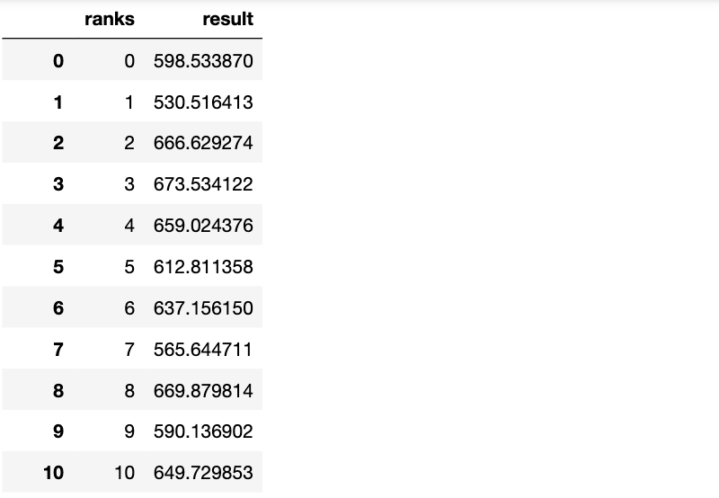
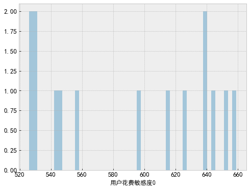
watch_feat='User fee sensitivity'
df_data[watch_feat].value_counts()
#4    29838
#5    21011
#2    20622
#3    20578
#1     7913
#0       38
#Name: user fee sensitivity, dtype: int64
for v in df_data[watch_feat].unique():
    plt.subplots(figsize=(8,6))
    sns.distplot(df_data.loc[df_data[watch_feat]==v,'Credit score'].values,bins=50,kde=False)
    plt.xlabel('User spending sensitivity{}'.format(v),fontsize=12)

import seaborn as sns
f, ax = plt.subplots(figsize=(20, 6))
sns.distplot(df_train['Last payment amount of payer (yuan)'].values, color='r', bins=50, kde=False)
plt.show()

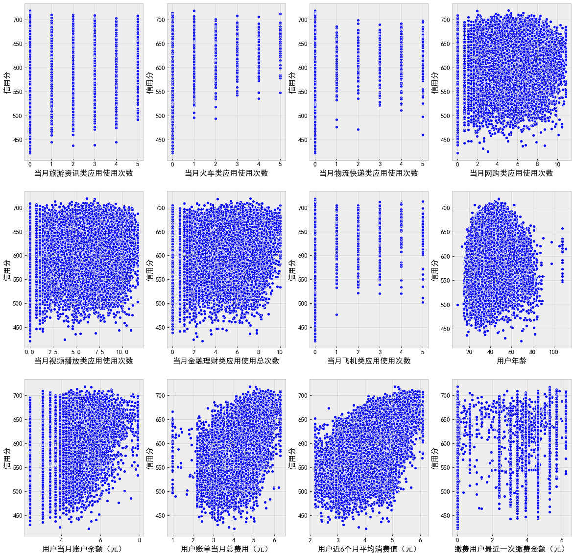
import seaborn as sns
name_list = ['Usage times of tourism information applications in the current month', 'Number of train applications used in the current month', 'Usage times of logistics express applications in the current month', 'Usage times of online shopping applications in the current month',
             'Application video playback times in the current month', 'Total usage times of financial management applications in the current month', 'Number of aircraft applications used in the current month', 'User age',
             'User's current month account balance (yuan)', 'Total cost of user bill in the current month (yuan)', 'Average consumption value of users in recent 6 months (yuan)', 'Last payment amount of payer (yuan)']

f, ax = plt.subplots(3, 4, figsize=(20, 20))

for i,name in enumerate(name_list):     
    sns.scatterplot(data=df_data, x=name, y='Credit score', color='b', ax=ax[i // 4][i % 4])
plt.show()

f, ax = plt.subplots(1, 3, figsize=(20, 6))

sns.kdeplot(data=df_data['Number of aircraft applications used in the current month'], color='r', shade=True, ax=ax[0])
sns.kdeplot(data=df_data['Number of train applications used in the current month'], color='c', shade=True, ax=ax[1])
sns.kdeplot(data=df_data['Usage times of tourism information applications in the current month'], color='b', shade=True, ax=ax[2])
plt.show()

""" Discrete feature analysis """
f, ax = plt.subplots(1, 2, figsize=(20, 6))
sns.boxplot(data=df_data, x='Time since the user last paid (month)', y='Credit score', ax=ax[0])
sns.boxplot(data=df_data, x='Is the paying user in arrears', y='Credit score', ax=ax[1])
plt.show()

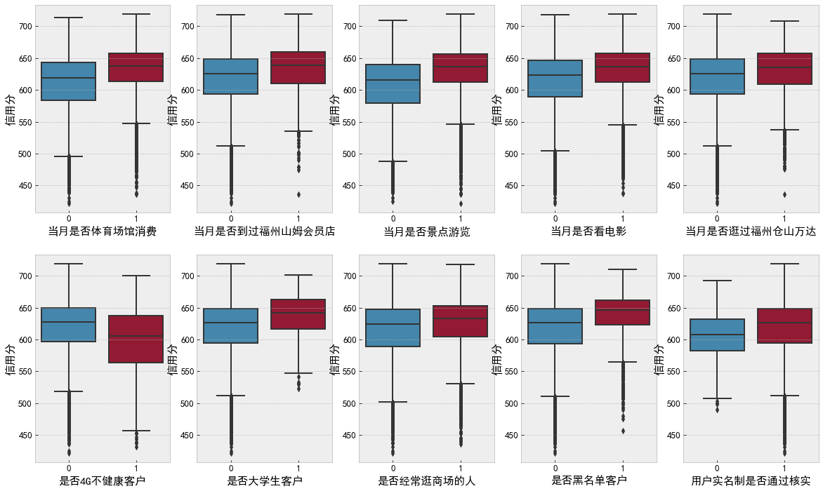
name_list = ['Whether the consumption of stadiums and Gymnasiums in the current month', 'Have you ever been to Fuzhou Sam's club in that month', 'Whether to visit scenic spots in the current month', 'Do you watch movies that month', 'Have you visited Fuzhou Cangshan Wanda in that month', 
             'Whether 4 G Unhealthy customers', 'Is it a college student customer', 'Do you often go shopping', 'Blacklisted customers', 'Whether the user's real name system has been verified']

f, ax = plt.subplots(2, 5, figsize=(20, 12))

for i,name in enumerate(name_list):
    sns.boxplot(data=df_data, x=name, y='Credit score', ax=ax[i // 5][i % 5])
plt.show()

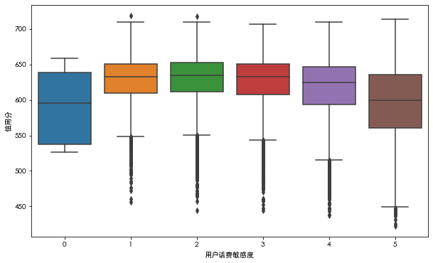
f, ax = plt.subplots(figsize=(10, 6))
sns.boxplot(data=df_data, x='User fee sensitivity', y='Credit score', ax=ax)
plt.show()

Data preprocessing involves many contents, including feature engineering, which is the largest part of the task. In order to make you read more clearly, the following lists some methods to be used in the processing part.

Data cleaning: missing value, abnormal value and consistency;
Feature coding: one hot and label coding;
Feature box: equal frequency, equal distance, clustering, etc
Derived variables: strong interpretability, suitable for model input;
Feature selection: variance selection, chi square selection, regularization, etc;

Finalized primary exploration engineering code

df_data[df_data['Number of communication circles in the current month'] > 1750].index
#Int64Index([], dtype='int64')
""" 
Why only cancel the tailing of one feature? Why keep the tailing of other features? Even if the score is increased offline, it is necessary
 Reserved. This is because offline, such as shopping mall tailing data, may be security guards in the real scene
 There may be only one security guard in the training set, so the offline verification will be improved after it is removed, but in the test set
 There is also a security guard in the test set. If the tail is lost, the security credit score accuracy of the test set will eventually be reduced 
"""
    
df_data.drop(df_data[df_data['Number of communication circles in the current month'] > 1750].index, inplace=True)
df_data.reset_index(drop=True, inplace=True)


""" 0 replace np.nan，Through offline verification, it is found that the number of missing values in the actual situation of data is greater than the number of 0 values, np.nan Better restore data authenticity """
na_list = ['User age', 'Last payment amount of payer (yuan)', 'Average consumption value of users in recent 6 months (yuan)','Total cost of user bill in the current month (yuan)']
for na_fea in na_list:
    df_data[na_fea].replace(0, np.nan, inplace=True)

### Cross validation
    
""" The call sensitivity is replaced by 0. Through offline verification, it is found that it is replaced by the median energy ratio np.nan Better restore data authenticity """
df_data['User fee sensitivity'].replace(0, df_data['User fee sensitivity'].mode()[0], inplace=True)


### Cross validation

Conclusion: by observing the discrete characteristics for many times, we can deepen our understanding of the data. For example, the user's call fee sensitivity characteristics are not directly generated by the user in the real world, but generated by the calculation of the specific association model of China Mobile, which can reverse the association degree of the user's credit to a great extent. In the box diagram, the user sensitivity presents a Gaussian distribution, which is in line with our conjecture about the business scenario.

Intermediate feature exploration (data pre Engineering)

Through the primary feature exploration, we can deepen our understanding of the data and realize the preliminary data preprocessing. Next, we begin to analyze the impact of features and features on credit score and carry out relevant intermediate feature exploration. Intermediate feature exploration is generally based on business scenarios, but as a novice, you can simply rely on your feelings to analyze the related features in the competition.

f, ax = plt.subplots(figsize=(20, 6))
sns.boxenplot(data=df_data, x='Have you visited Fuzhou Cangshan Wanda in that month', y='Credit score', hue='Have you ever been to Fuzhou Sam's club in that month', ax=ax)
plt.show()

""" Discrete exploration """
f, [ax0, ax1, ax2, ax3, ax4] = plt.subplots(1, 5, figsize=(20, 6))

sns.boxplot(data=df_data, x='Have you visited Fuzhou Cangshan Wanda in that month', y='Credit score', hue='Do you often go shopping', ax=ax0)
sns.boxplot(data=df_data, x='Have you ever been to Fuzhou Sam's club in that month', y='Credit score', hue='Do you often go shopping', ax=ax1)
sns.boxplot(data=df_data, x='Do you watch movies that month', y='Credit score', hue='Do you often go shopping', ax=ax2)
sns.boxplot(data=df_data, x='Whether to visit scenic spots in the current month', y='Credit score', hue='Do you often go shopping', ax=ax3)
sns.boxplot(data=df_data, x='Whether the consumption of stadiums and Gymnasiums in the current month', y='Credit score', hue='Do you often go shopping', ax=ax4)
plt.show()

""" Continuous exploration """
f, ax = plt.subplots(1, 2, figsize=(20, 6))

sns.scatterplot(data=df_data, x='Total cost of user bill in the current month (yuan)', y='Credit score', color='b', ax=ax[0])
sns.scatterplot(data=df_data, x='User's current month account balance (yuan)', y='Credit score', color='r', ax=ax[1])
plt.show()

f, ax = plt.subplots(1, 2, figsize=(20, 6))

sns.scatterplot(data=df_data, x='Total cost of user bill in the current month (yuan)', y='Credit score', color='b', ax=ax[0])
sns.scatterplot(data=df_data, x='Average consumption value of users in recent 6 months (yuan)', y='Credit score', color='r', ax=ax[1])
plt.show()

f, [ax0, ax1, ax2, ax3] = plt.subplots(1, 4, figsize=(20, 6))
sns.scatterplot(data=df_data, x='Usage times of online shopping applications in the current month', y='Credit score', hue='Do you often go shopping', ax=ax0)
sns.scatterplot(data=df_data, x='Usage times of logistics express applications in the current month', y='Credit score', hue='Do you often go shopping', ax=ax1)
sns.scatterplot(data=df_data, x='Total usage times of financial management applications in the current month', y='Credit score', hue='Do you often go shopping', ax=ax2)
sns.scatterplot(data=df_data, x='Application video playback times in the current month', y='Credit score', hue='Do you often go shopping', ax=ax3)
plt.show()

f, [ax0, ax1, ax2, ax3] = plt.subplots(1, 4, figsize=(20, 6))
sns.scatterplot(data=df_data, x='Number of aircraft applications used in the current month', y='Credit score', hue='Do you often go shopping', ax=ax0)
sns.scatterplot(data=df_data, x='Number of train applications used in the current month', y='Credit score', hue='Do you often go shopping', ax=ax1)
sns.scatterplot(data=df_data, x='Usage times of tourism information applications in the current month', y='Credit score', hue='Do you often go shopping', ax=ax2)
sns.scatterplot(data=df_data, x='User network age (month)', y='Credit score', hue='Do you often go shopping', ax=ax3)
plt.show()

Final intermediate exploration engineering Code:

""" x / (y + 1) Avoid infinity Inf，Gaussian smoothing + 1 """
df_data['Stable telephone charges'] = df_data['Total cost of user bill in the current month (yuan)'] / (df_data['User's current month account balance (yuan)'] + 1)
df_data['Relatively stable'] = df_data['Total cost of user bill in the current month (yuan)'] / (df_data['Average consumption value of users in recent 6 months (yuan)'] + 1)
df_data['Stable payment'] = df_data['Last payment amount of payer (yuan)'] / (df_data['Average consumption value of users in recent 6 months (yuan)'] + 1)

df_data['Have you ever been to a luxury mall in that month'] = (df_data['Have you visited Fuzhou Cangshan Wanda in that month'] + df_data['Have you ever been to Fuzhou Sam's club in that month']).map(lambda x: 1 if x > 0 else 0)
df_data['Total application usage'] = df_data['Usage times of online shopping applications in the current month'] + df_data['Usage times of logistics express applications in the current month'] + df_data['Total usage times of financial management applications in the current month'] + df_data['Application video playback times in the current month'] + df_data['Number of aircraft applications used in the current month'] + df_data['Number of train applications used in the current month'] + df_data['Usage times of tourism information applications in the current month']

Conclusion: through a large number of intermediate exploration, we can deepen the correlation between data. When conducting intermediate exploration, we should conduct offline stable verification test combined with the model. In some structured competitions, we can enter 10% in the competition through a large number of intermediate exploration.

Advanced feature exploration (data true scene)

In the data competition, if you want to win a high ranking or even a medal, you need not only a solid foundation of Feature Engineering, but also a deep business understanding of the data and be able to mine and extract the information hidden in the data. Next, I will explore the advanced features of the competition.

1. Interpret the feature itself from a business perspective and extract key information

Through the mining of the source of the feature, we observed the last payment amount (yuan) feature of payment users from a business perspective, and found that this feature has important hidden meaning. For example, some users do not have payment amount information, and some payment amounts have single digits. When there is an amount, payment users may pay through the Internet, automatic payment machines and other means, Finally, we extract the characteristics of user payment methods according to the above analysis.

count:100000.000000
mean: 53.721932
std: 62.214807
min: 0.000000
25%: 0.000000
50%: 49.900000
75%: 99.800000
max:1000.000000
name: last payment amount of payer (yuan), dtype:float64

df_data['Payment method'] = 0
df_data.loc[(df_data['Last payment amount of payer (yuan)'] != 0) & (df_data['Last payment amount of payer (yuan)'] % 10 == 0), 'Payment method'] = 1
df_data.loc[(df_data['Last payment amount of payer (yuan)'] != 0) & (df_data['Last payment amount of payer (yuan)'] % 10 > 0), 'Payment method'] = 2

f, ax = plt.subplots(figsize=(20, 6))
sns.boxplot(data=df_data, x='Payment method', y='Credit score', ax=ax)
plt.show()

2. Make full use of external information to make the features have practical scene significance

By browsing a large number of star credit sub data of China Mobile and according to the package information on China Mobile's official website, we extract and classify the characteristics of users' network age.

df_data['Credit qualification'] = df_data['User network age (month)'].apply(lambda x: 1 if x > 12 else 0)
f, ax = plt.subplots(figsize=(10, 6))
sns.boxenplot(data=df_data, x='Credit qualification', y='Credit score', ax=ax)
plt.show()

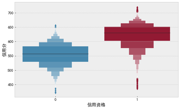
3. Make full use of the information on the official website and actively contact the sponsor for data business problems

After interpreting the title of the official website of the competition in detail for many times, we extracted the proportion of user sensitivity according to the characteristic information provided by the official website of the competition.

The first level of user fee sensitivity indicates that the sensitivity level is the largest
According to the results of extreme value calculation method and leaf index weight, the sensitivity level of sensitive users is generated according to the rules:

First, sort the sensitivity users in descending order according to the middle score:

The sensitivity level of the top 5% of users is level 1
The sensitivity level of the next 15% of users is level 2;
The sensitivity level of the next 15% of users is level 3;
The sensitivity level of the next 25% of users is level 4;
The sensitivity level of the last 40% of users is level 5;

df_data['Proportion of sensitivity'] = df_data['User fee sensitivity'].map({1:1, 2:3, 3:3, 4:4, 5:8})

f, ax = plt.subplots(1, 2, figsize=(20, 6))
sns.boxenplot(data=df_data, x='Proportion of sensitivity', y='Credit score', ax=ax[0])
sns.boxenplot(data=df_data, x='User fee sensitivity', y='Credit score', ax=ax[1])
plt.show()

Conclusion: in the advanced exploration stage, engineers are always more sensitive than students. Of course, talents will also be displayed here. The most important thing in the data competition is to make promising efforts!

Algorithm model

In structured competitions, the commonly used models of machine learning include LGB, XGB, CAT and other models. The algorithm is fast and can accommodate missing values. Because we have extracted missing values and clarified the business significance of missing values before, we use LGB as the training model.

model data

lab = 'Credit score'
X = df_data.loc[df_data[lab].notnull(), (df_data.columns != lab) & (df_data.columns != 'User code')]
y = df_data.loc[df_data[lab].notnull()][lab]
X_pred = df_data.loc[df_data[lab].isnull(), (df_data.columns != lab) & (df_data.columns != 'User code')]
df_data.head()

model parameter

""" The model parameters are the author's ancestral parameters """
lgb_param_l1 = {
    'learning_rate': 0.01, #Step of gradient descent
    'boosting_type': 'gbdt',#Gradient lifting decision tree
    'objective': 'regression_l1', #Task objective (L1 loss, alias=mean_absolute_error, mae)
    'metric': 'mae',
    'min_child_samples': 46,# The minimum amount of data on a leaf
    'min_child_weight': 0.01,
    'feature_fraction': 0.6,#Select the first 60% of the features in each iteration
    'bagging_fraction': 0.8,#Select some data randomly without resampling
    'bagging_freq': 2, #bagging is performed every 2 iterations
    'num_leaves': 31,#Number of leaves on a tree
    'max_depth': 5,#Maximum depth of tree
    'lambda_l2': 1, # Represents L2 regularization
    'lambda_l1': 0,# Represents L1 regularization
    'n_jobs': -1,
    'seed': 4590,
}

Model framework

In the actual fierce competition, the number of submissions is always limited, so players must build a reasonable offline verification framework. In this competition, in order to ensure the accuracy of offline verification, I choose 50% cross verification, which can well avoid over fitting.

from sklearn.model_selection import KFold
import lightgbm as lgb

y_counts = 0
y_scores = np.zeros(5)
y_pred_l1 = np.zeros([5, X_pred.shape[0]])#[5,50000]
y_pred_all_l1 = np.zeros(X_pred.shape[0])#[50000,]

for n in range(1): # 0
    kfold = KFold(n_splits=5, shuffle=True, random_state=2019 + n)
    kf = kfold.split(X, y)

    for i, (train_iloc, test_iloc) in enumerate(kf):
        #print(len(test_iloc))
        print("{},".format(i + 1), end='')
        X_train, X_test, y_train, y_test = X.iloc[train_iloc, :], X.iloc[test_iloc, :], y[train_iloc], y[test_iloc]
        lgb_train = lgb.Dataset(X_train, y_train)
        lgb_valid = lgb.Dataset(X_test, y_test, reference=lgb_train)
        lgb_model = lgb.train(train_set=lgb_train, valid_sets=lgb_valid, 
                              params=lgb_param_l1, num_boost_round=6000, verbose_eval=-1, early_stopping_rounds=100)

        y_scores[y_counts] = lgb_model.best_score['valid_0']['l1']
        y_pred_l1[y_counts] = lgb_model.predict(X_pred, num_iteration=lgb_model.best_iteration)#Forecast credit score
        y_pred_all_l1 += y_pred_l1[y_counts] 
        y_counts += 1
        #print(y_pred_l1)
y_pred_all_l1 /= y_counts
print(y_scores, y_scores.mean())
#1,Training until validation scores don't improve for 100 rounds.
#Early stopping, best iteration is:
#[2555]	valid_0's l1: 14.6827
#2,Training until validation scores don't improve for 100 rounds.
#Early stopping, best iteration is:
#[3616]	valid_0's l1: 14.4936
#3,Training until validation scores don't improve for 100 rounds.
#Early stopping, best iteration is:
#[2196]	valid_0's l1: 14.8204
#4,Training until validation scores don't improve for 100 rounds.
#Early stopping, best iteration is:
#[3355]	valid_0's l1: 14.6649
#5,Training until validation scores don't improve for 100 rounds.
#Early stopping, best iteration is:
#[3195]	valid_0's l1: 14.7147
#[14.68266276 14.49360643 14.82035007 14.66492709 14.71471457] 14.675252185621542