This article will summarize the time series prediction methods, introduce all methods in categories and provide corresponding python code examples. The following is the list of methods to be introduced in this article:
1. Time series prediction using smoothing technique
- exponential smoothing
- Holt winters method
2. Univariate time series prediction
- Autoregressive (AR)
- Moving average model (MA)
- Autoregressive moving average model (ARMA)
- Differential integrated moving average autoregressive model (ARIMA)
- Seasonal ARIMA (SARIMA)
3. Time series prediction of exogenous variables
- Sarimax with exogenous variables (sarimax)
- Vector autoregressive moving average with exogenous regressors (VARMAX)
4. Multivariate time series prediction
- Vector autoregressive (VAR)
- Vector autoregressive moving average (VARMA)
Let's introduce the above methods one by one and give a code example of python
1. Exponential Smoothing
Exponential smoothing method is the weighted average value of past observations. As the observations get older, the weight will decay exponentially. In other words, the closer the observation time, the higher the correlation weight. It can quickly generate reliable predictions and is suitable for a wide range of time series.
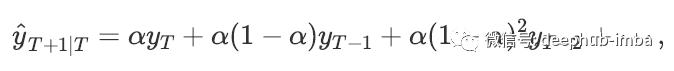
Simple exponential smoothing: this method is suitable for predicting univariate time series data without clear trend or seasonal pattern. The simple exponential smoothing method models the next time step as an exponentially weighted linear function of the observations of the previous time step.
It requires a parameter called alpha (a), also known as smoothing factor or smoothing coefficient, which controls the rate at which the influence of the observed value of the previous time step decays exponentially, that is, the rate at which the weight decreases. A is usually set to a value between 0 and 1. A larger value means that the model focuses on recent past observations, while a smaller value means that more history will be considered when making predictions. The simple mathematical explanation of simple exponential smoothing time series is as follows:
# SES
from statsmodels.tsa.holtwinters import SimpleExpSmoothing
from random import random
# contrived dataset
data = [x + random() for x in range(1, 100)]
# fit model
model = SimpleExpSmoothing(data)
model_fit = model.fit()
# make prediction
yhat = model_fit.predict(len(data), len(data))
print(yhat)
2. Holt winters method
In early 1957, Holt extended the simple exponential smoothing method to predict trend data. This method, called Holt linear trend, includes a prediction equation and two smoothing equations (one for level and one for trend) and corresponding smoothing parameters α And β. Later, in order to avoid infinite repetition of trend patterns, the damped trend method was introduced. When many sequences need to be predicted, it proved to be a very successful and most popular single method. In addition to two smoothing parameters, it also includes a parameter called damping φ Additional parameters for.
Once the trend can be captured, the Holt winters method extends the traditional Holt method to capture seasonality. Holt winters' seasonal method includes prediction equation and three smoothing equations - one for level, one for trend and one for seasonal component, with corresponding smoothing parameters α,β And γ.
There are two variants of this method, which differ in the nature of seasonal components. When the seasonal change is approximately constant in the whole series, the addition method is preferred, while when the seasonal change is proportional to the series level, the multiplication method is preferred.
# HWES
from statsmodels.tsa.holtwinters import ExponentialSmoothing
from random import random
# contrived dataset
data = [x + random() for x in range(1, 100)]
# fit model
model = ExponentialSmoothing(data)
model_fit = model.fit()
# make prediction
yhat = model_fit.predict(len(data), len(data))
print(yhat)
3. Autoregressive (AR)
In the AR model, we use the linear combination of past values of variables to predict the variables of interest. The term autoregression indicates that it is the regression of variables to themselves. The simple mathematical expression of AR model is as follows:
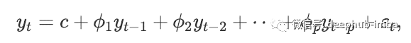
here, ε t is white noise. This is similar to multiple regression, but uses the lag value of yt as the prediction variable. We call it AR(p) model, that is, p-order autoregressive model.
#AR

from statsmodels.tsa.ar_model import AutoReg
from random import random
# contrived dataset
data = [x + random() for x in range(1, 100)]
# fit model
model = AutoReg(data, lags=1)
model_fit = model.fit()
# make prediction
yhat = model_fit.predict(len(data), len(data))
print(yhat)
4. Moving average model (MA)
Unlike AR models that use the past values of predictive variables in regression, Ma models focus on past prediction errors or residuals in models similar to regression. The simple mathematical expression of MA model is as follows:
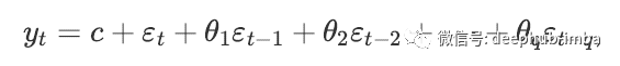
here, ε t is white noise. We call it MA(q) model, that is, q-order moving average model.
# MA
from statsmodels.tsa.arima.model import ARIMA
from random import random
# contrived dataset
data = [x + random() for x in range(1, 100)]
# fit model
model = ARIMA(data, order=(0, 0, 1))
model_fit = model.fit()
# make prediction
yhat = model_fit.predict(len(data), len(data))
print(yhat)
It should be noted that the moving average method mentioned here should not be confused with calculating the moving average of time series, because they are different concepts.
5. Autoregressive moving average model (ARMA)
In the AR model, we use the linear combination of the past value of the variable and the past prediction error or residual to predict the variable of interest. It combines autoregressive (AR) and moving average (MA) models.
The AR part involves regression of the lag (i.e. past) value of the variable itself. The Ma part involves modeling the error term as a linear combination of error terms that occurred simultaneously at different times in the past. The notation of the model involves specifying the order of AR(p) and MA(q) models as parameters of the ARMA function, such as ARMA (p, q). The simple mathematical representation of ARMA model is as follows:

# ARMA
from statsmodels.tsa.arima.model import ARIMA
from random import random
# contrived dataset
data = [random() for x in range(1, 100)]
# fit model
model = ARIMA(data, order=(2, 0, 1))
model_fit = model.fit()
# make prediction
yhat = model_fit.predict(len(data), len(data))
print(yhat)
6. Differential integrated moving average autoregressive model (ARIMA)
If we combine difference with autoregressive and moving average models, we will obtain ARIMA model. Arima is the acronym of Autoregressive Integrated Moving Average model. It combines autoregressive (AR) and moving average model (MA) and the differential preprocessing process of the sequence in order to make the sequence stable. This process is called integral (I). The simple mathematical expression of ARIMA model is as follows:

Where y ′ t is the number of differential grades. The "prediction variable" on the right includes lag value and lag error. We call it ARIMA(p,d,q) model.
Here, p is the order of the autoregressive part, d is the first-order difference degree involved, and q is the order of the moving average part.
Significance of ACF and PACF diagrams in finding order p and q:
- In order to find the order p of AR(p) model: we expect that the ACF diagram will gradually decrease, and the PACF will decrease or cut off sharply after P lags significantly.
- In order to find the order p of MA(q) model: we expect that the PACF diagram will gradually decrease, and the ACF should decrease or cut off sharply after some significant lag of Q.
# ARIMA
from statsmodels.tsa.arima.model import ARIMA
from random import random
# contrived dataset
data = [x + random() for x in range(1, 100)]
# fit model
model = ARIMA(data, order=(1, 1, 1))
model_fit = model.fit()
# make prediction
yhat = model_fit.predict(len(data), len(data), typ='levels')
print(yhat)
7. Seasonal ARIMA (SARIMA)
ARIMA model can also model a wide range of seasonal data. Seasonal ARIMA model is formed by including additional seasonal items in ARIMA model.
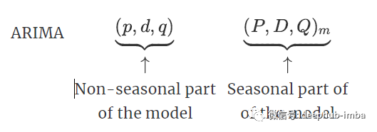
Here, m = number of steps per time season. We use uppercase symbols for seasonal parts of the model and lowercase symbols for non seasonal parts of the model.
It combines ARIMA models with the ability to perform the same autoregressive, differential and moving average modeling at the seasonal data level.
# SARIMA
from statsmodels.tsa.statespace.sarimax import SARIMAX
from random import random
# contrived dataset
data = [x + random() for x in range(1, 100)]
# fit model
model = SARIMAX(data, order=(1, 1, 1), seasonal_order=(0, 0, 0, 0))
model_fit = model.fit(disp=False)
# make prediction
yhat = model_fit.predict(len(data), len(data))
print(yhat)
8. SARIMA (SARIMAX) with exogenous variables
SARIMAX model is an extension of the traditional SARIMA model, including the modeling of exogenous variables. It is the abbreviation of seasonal autorepressant integrated moving average with exogenous regressors
Exogenous variables are variables whose values are determined outside the model and applied to the model. They are also called covariates. The observations of exogenous variables are directly included in the model at each time step, and the modeling method is different from the use of main endogenous sequences.
The SARIMAX method can also be used to simulate other changes with exogenous variables by including exogenous variables, such as ARX, MAX, ARMAX and ARIMAX.
# SARIMAX
from statsmodels.tsa.statespace.sarimax import SARIMAX
from random import random
# contrived dataset
data1 = [x + random() for x in range(1, 100)]
data2 = [x + random() for x in range(101, 200)]
# fit model
model = SARIMAX(data1, exog=data2, order=(1, 1, 1), seasonal_order=(0, 0, 0, 0))
model_fit = model.fit(disp=False)
# make prediction
exog2 = [200 + random()]
yhat = model_fit.predict(len(data1), len(data1), exog=[exog2])
print(yhat)
9. Vector autoregressive (VAR)
VAR model is a generalization of univariate autoregressive model, which is used to predict time series vector or multiple parallel time series, such as multivariate time series. It is an equation about each variable in the system.
If the series are stationary, they can be predicted by fitting var directly to the data (called "VAR in levels"). If the sequence is non-stationary, we will take the difference of the data to make it stationary, and then fit the VAR model (called "VAR in differences").
We call it p-order VAR model.
# VAR
from statsmodels.tsa.vector_ar.var_model import VAR
from random import random
# contrived dataset with dependency
data = list()
for i in range(100):
    v1 = i + random()
    v2 = v1 + random()
    row = [v1, v2]
    data.append(row)
# fit model
model = VAR(data)
model_fit = model.fit()
# make prediction
yhat = model_fit.forecast(model_fit.y, steps=1)
print(yhat)
10. Vector autoregressive moving average model (VARMA)
VARMA method is the generalization of ARMA to multiple parallel time series, such as multivariate time series. The finite order VAR process with finite order MA error term is called VARMA.
The formula of the model specifies the order of AR(p) and MA(q) models as the parameters of the VARMA function, such as VARMA (p, q). VARMA models can also be used for VAR or VMA models.
# VARMA
from statsmodels.tsa.statespace.varmax import VARMAX
from random import random
# contrived dataset with dependency
data = list()
for i in range(100):
    v1 = random()
    v2 = v1 + random()
    row = [v1, v2]
    data.append(row)
# fit model
model = VARMAX(data, order=(1, 1))
model_fit = model.fit(disp=False)
# make prediction
yhat = model_fit.forecast()
print(yhat)
11. Vector autoregressive moving average model with exogenous variables (VARMAX)
Vector autorepression moving average with exogenous regressors (varmax) is an extension of the VARMA model, which also includes modeling using exogenous variables. It is the generalization of ARMAX method to multiple parallel time series, that is, the multivariable version of ARMAX method.
The VARMAX method can also be used to model inclusion models containing exogenous variables, such as VARX and VMAX.
# VARMAX
from statsmodels.tsa.statespace.varmax import VARMAX
from random import random
# contrived dataset with dependency
data = list()
for i in range(100):
    v1 = random()
    v2 = v1 + random()
    row = [v1, v2]
    data.append(row)
data_exog = [x + random() for x in range(100)]
# fit model
model = VARMAX(data, exog=data_exog, order=(1, 1))
model_fit = model.fit(disp=False)
# make prediction
data_exog2 = [[100]]
yhat = model_fit.forecast(exog=data_exog2)
print(yhat)
summary
In this article, it basically covers all the major time series prediction problems. We can organize the methods mentioned above into the following important directions:
- AR: autoregressive
- MA: average movement
- 1: Differential integration
- S: Seasonality
- 5: V ector (multidimensional input)
- 10: Exogenous variable
Each algorithm mentioned in this paper is basically a combination of these methods. This paper has focused on the description and code demonstration of each algorithm. If you want to know more about it, please check the relevant papers.
https://www.overfit.cn/post/48b9c34c2b8c4a938e838d3c3616e789