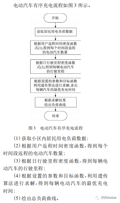
1 Introduction
In order to ensure that the transformer is not overloaded when charging the electric vehicle in the community, an orderly charging control method of the electric vehicle in the community based on genetic algorithm is proposed On the basis of comprehensively considering the charging demand of users, aiming at not changing the power supply capacity of transformer and "cutting peak and filling valley", Monte Carlo method is used to simulate the load, and genetic algorithm is used to solve the optimal charging time of electric vehicles, so as to realize the orderly charging of electric vehicles in the community The analysis results show that compared with disordered charging, the proposed method can meet the charging needs of users without changing the power supply capacity of the transformer, and effectively realize "peak cutting and valley filling"
Genetic algorithm is an optimization algorithm that imitates the biological evolution mechanism in nature. Compared with other optimization algorithms, it has the advantages of good convergence and fast calculation time. The steps of genetic algorithm are as follows:
(1) set the initial parameters, generate the initial population, and calculate the fitness of each individual;
(2) select the individual with good fitness for the next operation;
(3) when the random variable is less than the crossover probability of genetic algorithm, the individual will perform crossover operation to generate a new population;
(4) when the random variable is less than the mutation probability of genetic algorithm, the individual will mutate;
(5) judge the new species group, eliminate the invalid individuals and retain the individuals with good fitness. The number of iterations increases once and returns (2).
Monte Carlo method is a statistical simulation method, which mainly obtains the results by establishing a model and setting conditions for a large number of random sampling. In this paper, Monte Carlo method is used to simulate the disordered charging process of electric vehicle. The steps of Monte Carlo method are as follows:
(1) set the number of electric vehicles and establish the load model in Section 1.1;
(2) generate user return time, daily mileage and other data of each electric vehicle;
(3) calculate the charging time period and charging load of each electric vehicle;
(4) generate disordered charging load curve.
Part 2 code
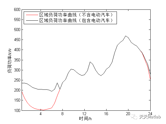
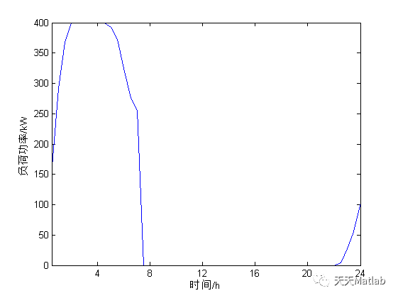
%%------------------------------------------------------%Genetic algorithm is used to optimize the orderly charging of electric vehicles; The optimization objectives include the lowest charging cost and the required charging time (the electric vehicle is charged with enough electricity)%Considering the influence of electric vehicle charging on power grid load, the peak valley difference of load is minimized.%--------------------------------------------------------clcclearwarning off%Real time electricity price, data import, data source PJMRP=[3.10000000000000,3.05000000000000,3,2.80000000000000,2.60000000000000,2.55000000000000,2.50000000000000,2.60000000000000,2.70000000000000,2.80000000000000,2.90000000000000,3.20000000000000,3.50000000000000,3.60000000000000,3.70000000000000,3.67500000000000,3.65000000000000,3.70000000000000,3.75000000000000,3.82500000000000,3.90000000000000,3.92500000000000,3.95000000000000,4.02500000000000,4.10000000000000,4.15000000000000,4.20000000000000,4.20500000000000,4.21000000000000,4.28000000000000,4.35000000000000,4.42500000000000,4.50000000000000,4.60000000000000,4.70000000000000,4.62000000000000,4.54000000000000,4.39500000000000,4.25000000000000,4.22500000000000,4.20000000000000,4.05000000000000,3.90000000000000,3.60000000000000,3.30000000000000,3.20000000000000,3.10000000000000,3.10000000000000];Price=[RP(35:48),RP(1:14)];% Set vehicle daily 17:00 Then go home to recharge; Leave home after 7 o'clock every day without charging Num=100;%Number of electric vehicles PEV=4;global PEV% load SOC_startSOC_start=normrnd(0.3,0.05,1,Num);global SOC_startSOC_end=0.95*ones(1,Num);global SOC_endC=35; global Cnumber=Num;%Number of individuals in the population%% Genetic algorithm parameter setting NP=300;% Total number of initial populations NG=80 ;% Total number of iterations Pc=0.8; Pm=0.4;% Variation rate COUNTER=10;%% Generate initial population for i=1:NP data(i).Initial=Initial(number); data(i).generation=data(i).Initial;end%% Calculate initial population fitness for i=1:NP data(i).Fitness=Fitness(data(i).generation,PEV,Price,SOC_start,SOC_end,C);endintinial_Fitness_1=max([data(:).Fitness]);%% Carry out heredity, crossover and variation maxium_Fitness=[];temp_Fitness=intinial_Fitness_1;for k=1:NG sum_Fitness=sum([data(1:NP).Fitness]); %Sum of all individual fitness values Px = [data(1:NP).Fitness]/sum_Fitness; %Average of all individual fitness values PPx = 0; PPx(1) = Px(1); for i=2:NP %Probability accumulation for roulette strategy PPx(i) = PPx(i-1) + Px(i); end for i=1:NP sita = rand(); for n=1:NP if sita <= PPx(n) SelFather = n; %Father determined according to roulette strategy break; end end Selmother = floor(rand()*(NP-1))+1; %Random selection of mothers posCut = floor(rand()*(number-2)) + 1; %Randomly determine the intersection r1 = rand(); %% overlapping if r1<=Pc %Pc Is the crossover rate %% COUNTER Number of elites for temp_count=1:COUNTER posCut = floor(rand()*(number-2)) + 1; TEMP(temp_count).generation(:,1:posCut) = data(SelFather).generation(:,1:posCut); TEMP(temp_count).generation(:,(posCut+1):number) = data(Selmother).generation(:,(posCut+1):number); end TEMP(COUNTER+1).generation=data(SelFather).generation; TEMP(COUNTER+2).generation=data(Selmother).generation; for temp_count=1:COUNTER TEMP(temp_count).Fitness=Fitness(TEMP(temp_count).generation,PEV,Price,SOC_start,SOC_end,C); end [TEMP_Fitness,Location]=max([TEMP(:).Fitness]); data1(i).generation=TEMP(Location).generation; %% % data1(i).generation(:,1:posCut) = data(SelFather).generation(:,1:posCut);% data1(i).generation(:,(posCut+1):number) = data(Selmother).generation(:,(posCut+1):number); r2 = rand(); %% variation if r2 <= Pm % Pm Variation rate posMut = round(rand()*(number-1) + 1); for j=1:size(data1,2) data1(j).generation(:,posMut)=generate( data1(j).generation(:,posMut)); end end else data1(i).generation =data(SelFather).generation(:,:); end end %% choice for i=1:NP data(i).Fitness= Fitness(data(i).generation,PEV,Price,SOC_start,SOC_end,C); %Offspring fitness end for i=1:NP data1(i).Fitness= Fitness(data1(i).generation,PEV,Price,SOC_start,SOC_end,C); %Offspring fitness end [value1,index1]=sort([data(1:NP).Fitness],'descend'); [value2,index2]=sort([data1(1:NP).Fitness],'descend'); j=1; for i=index1(1:NP/2) temp_1(j).p=data(i).generation; j=j+1; end j=1; for i=index2(1:NP/2) temp_2(j).p=data1(i).generation; j=j+1; end for i=1:NP/2 data(i).generation =temp_1(i).p; end for i=1:NP/2 data(NP/2+i).generation =temp_2(i).p; end for i=1:NP data(i).Fitness= Fitness(data(i).generation,PEV,Price,SOC_start,SOC_end,C); %Offspring fitness end temp_Fitness=max([data(1:NP).Fitness]); maxium_Fitness=[maxium_Fitness;temp_Fitness];endFitness_initial= -inf;for i=1:NP if data(i).Fitness> Fitness_initial INDEX=i; %Take the best value in the individual as the final result Fitness_initial=data(i).Fitness; endend%% Visualization of genetic algorithm results figure(1) plot(-maxium_Fitness)% Draw the fitness of the best individual of each generation xlabel('Genetic algebra')ylabel('Combined objective function value')title('evolutionary process ')FITNESS_JY=-maxium_Fitness;save FITNESS_JYfigure(2)EV_load=sum(data(INDEX).generation');EV=[EV_load(15:end),zeros(1,20),EV_load(1:14)];plot(EV*PEV)set(gca, 'XLim',[1 48]); % X Data display range of axis set(gca, 'XTick',[8,16,24,32,40,48] ); % X Marking point of axis set(gca, 'XTicklabel',{'4','8','12','16','20','24'}); % X Mark of shaft xlabel('time/h')ylabel('Load power/kW')figure(3)Residential_load=[1962.55433333333,1617.09200000000,1397.80300000000,1240.56566666667,1139.44666666667,1087.19533333333,1047.75966666667,1039.21600000000,1025.50600000000,1055.46700000000,1082.60533333333,1130.10900000000,1361.02566666667,1719.95200000000,2047.19933333333,2384.35633333333,2527.08400000000,2849.10700000000,3038.91600000000,3026.13366666667,2888.03833333333,2787.28300000000,2730.16333333333,2762.67133333333,2965.20133333333,3403.65066666667,3292.44533333333,3011.74400000000,2804.51133333333,2717.41300000000,2834.95466666667,3040.08966666667,3160.87966666667,3381.25666666667,3864.43433333333,4218.04066666667,4372.06066666667,4467.65866666667,4694.08000000000,4610.18166666667,4374.74966666667,4266.39233333333,4200.47800000000,4027.01666666667,3845.33500000000,3510.83266666667,3183.25400000000,2515.23000000000]*0.1;plot(Residential_load,'r-');hold on% Local load curve plot(EV+Residential_load,'k-')% Local load curve after superposition of electric vehicles EV_JY=EV;save EV_JYset(gca, 'YLim',[100 600]); % X Data display range of axis set(gca, 'XLim',[1 48]); % X Data display range of axis set(gca, 'XTick',[8,16,24,32,40,48] ); % X Marking point of axis set(gca, 'XTicklabel',{'4','8','12','16','20','24'}); % X Mark of shaft xlabel('time/h')ylabel('Load power/kW')legend('Regional load power curve (excluding electric vehicle)','location','northwest','Regional load power curve (including electric vehicle)','location','northwest')3 simulation results
4 references
[1] Wang Jinfeng, Xie Shiyu, Li Junhao, et al Orderly charging strategy of community electric vehicles based on genetic algorithm [J] Low voltage apparatus, 2019, 000 (010): 47-50
Blogger profile: good at matlab simulation in intelligent optimization algorithm, neural network prediction, signal processing, cellular automata, image processing, path planning, UAV and other fields. Relevant matlab code problems can be exchanged through private letters.
Some theories cite online literature. If there is infringement, contact the blogger and delete it.