Outline of this paper:
Due to the large amount of content, this article will start directly from Chapter 5. For the complete version of the document, please click the link below:
Nanny level tutorial of data warehouse construction PDF document
The contents of the first four chapters are available at the link above
Chapter V core of real-time warehouse construction
1. Real time calculation
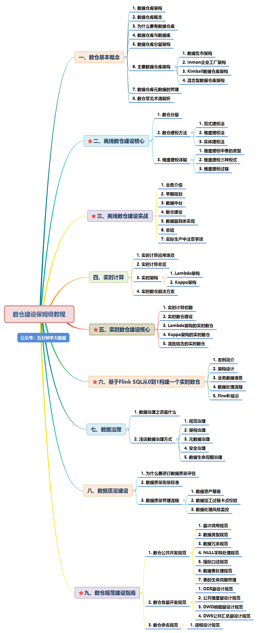
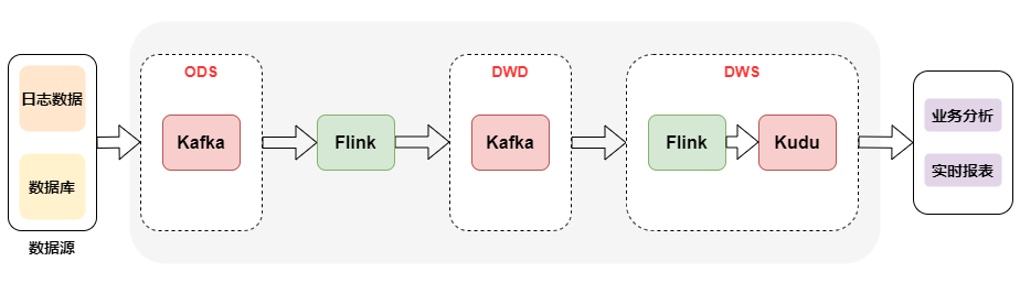
Although real-time computing has only become popular in recent years, some companies have the demand for real-time computing in the early stage, but the amount of data is relatively small, so a complete system can not be formed in real-time. Basically, all development is based on specific analysis of specific problems. One needs to do one, and the relationship between them is basically not considered. The development form is as follows:
As shown in the figure above, after obtaining the data source, it will undergo data cleaning, dimension expansion, business logic processing through Flink, and finally business output directly. Taking this link apart, the data source side will repeatedly reference the same data source, and then repeat the operations of cleaning, filtering and dimension expansion. The only difference is that the code logic of the business is different.
With the increasing demand of products and business personnel for real-time data, there are more and more problems in this development mode:
-
More and more data indicators, "chimney" development leads to serious code coupling problems.
-
There are more and more demands, some need detailed data, and some need OLAP analysis. A single development model is difficult to meet a variety of needs.
-
Every demand must apply for resources, which leads to the rapid expansion of resource cost and the intensive and effective utilization of resources.
-
Lack of a sound monitoring system, unable to find and fix problems before they have an impact on the business.
Let's look at the development and problems of real-time data warehouse, which is very similar to offline data warehouse. After the large amount of data in the later stage, various problems arise. How did offline data warehouse solve them at that time? Offline data warehouse decouples data through layered architecture, and multiple businesses can share data. Can real-time data warehouse also use layered architecture? Yes, of course, but there are still some differences between the details and offline layering, which will be discussed later.
2. Real time warehouse construction
In terms of methodology, real-time and off-line are very similar. In the early stage of off-line data warehouse, it is also a specific analysis of specific problems. When the data scale rises to a certain amount, we will consider how to manage it. Layering is a very effective way of data governance, so the first consideration is the layering processing logic on how to manage the real-time data warehouse.
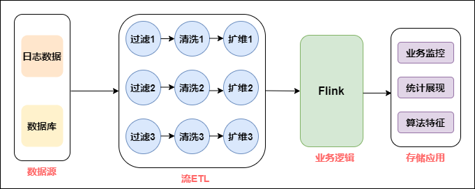
The architecture of real-time data warehouse is shown in the figure below:
From the above figure, we specifically analyze the role of each layer:
-
Data source: at the level of data source, offline and real-time data sources are consistent. They are mainly divided into log type and business type. Log type also includes user log, buried point log and server log.
-
Real time detail layer: in the detail layer, in order to solve the problem of repeated construction, it is necessary to build a unified basic detail data layer by using the mode of offline data warehouse, and manage it according to the theme. The purpose of the detail layer is to provide directly available data to the downstream. Therefore, it is necessary to carry out unified processing on the basic layer, such as cleaning, filtering, dimension expansion, etc.
-
Summary layer: the summary layer can directly calculate the results through Flink's concise operator and form a summary index pool. All indicators are processed in the summary layer. Everyone manages and constructs according to unified specifications to form reusable summary results.
We can see that the layers of real-time warehouse and offline warehouse are very similar, such as data source layer, detail layer, summary layer, and even application layer. Their naming patterns may be the same. However, it is not difficult to find many differences between the two:
-
Compared with offline data warehouse, real-time data warehouse has fewer levels:
-
From the current experience of building offline data warehouse, the content of the data detail layer of the data warehouse will be very rich, and the concept of mild summary layer is generally included in addition to the processing of detailed data. In addition, the application layer data in the offline data warehouse is inside the data warehouse, but in the real-time data warehouse, the app application layer data has fallen into the storage medium of the application system, so this layer can be separated from the table of the data warehouse.
-
Advantages of less application layer construction: when processing data in real time, each layer will inevitably produce a certain delay.
-
Advantages of less construction of the summary layer: when summarizing statistics, in order to tolerate the delay of some data, some artificial delays may be created to ensure the accuracy of the data. For example, when counting the data in order events related to cross day, you may wait until 00:00:05 or 00:00:10 to make sure that all the data before 00:00 have been accepted in place. Therefore, if there are too many layers in the summary layer, it will increase the artificial data delay.
-
-
Compared with offline data warehouse, the data source storage of real-time data warehouse is different:
- When building offline data warehouse, the whole offline data warehouse is basically based on Hive table. However, when building a real-time data warehouse, the same table will be stored in different ways. For example, in common cases, detailed data or summary data will be stored in Kafka, but dimensional information such as cities and channels need to be stored with the help of databases such as Hbase, MySQL or other KV storage.
3. Real time data warehouse of lambda architecture
The concept of Lambda and Kappa architecture has been explained in the previous article. If you don't understand it, you can click the link: Read and understand big data real-time computing
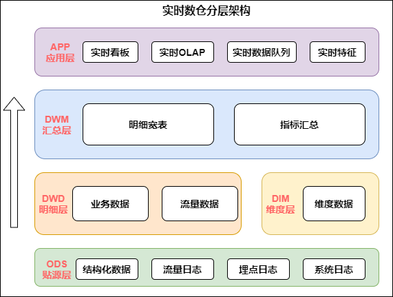
The following figure shows the specific practice of Lambda architecture based on Flink and Kafka. The upper layer is real-time computing, the lower layer is offline computing, which is divided horizontally by computing engine and vertically by real-time data warehouse:
Lambda architecture is a classic architecture. In the past, there were not many real-time scenes, mainly offline. When real-time scenes were added, due to the different timeliness of offline and real-time, the technical ecology was different. Lambda architecture is equivalent to adding a real-time production link to carry out an integration at the application level, two-way production and independent. This is also a logical way in business applications.
There will be some problems in two-way production, such as double processing logic, double development, operation and maintenance, and resources will also become two resource links. Because of the above problems, a Kappa architecture has evolved.
4. Real time data warehouse of kappa architecture
Kappa architecture is equivalent to Lambda architecture without offline computing, as shown in the figure below:
Kappa architecture is relatively simple in terms of architecture design and unified production. A set of logic produces offline and real-time at the same time. However, there are great limitations in the actual application scenario, because the same table of real-time data will be stored in different ways, which leads to the need to cross data sources during association, and there are great limitations in operating data. Therefore, there are few cases of direct production and landing with kappa architecture in the industry, and the scenario is relatively single.
Students who are familiar with real-time warehouse production may have a question about Kappa architecture. Because we often face business changes, many business logic needs to be iterated. If the caliber of some previously output data is changed, it needs to be recalculated or even redrawn the historical data. For real-time data warehouse, how to solve the problem of data recalculation?
The idea of Kappa architecture in this part is: first, prepare a message queue that can store historical data, such as Kafka, and this message queue can support you to restart consumption from a historical node. Then you need to start a new task and consume the data on Kafka from an earlier time node. Then, when the running progress of this new task can be equal to that of the running task, you can switch the downstream of the current task to the new task, and the old task can be stopped, And the result table of the original output can also be deleted.
5. Real time data warehouse with flow batch combination
With the development of real-time OLAP technology, the current open source OLAP engine has greatly improved in performance and ease of use, such as Doris, Presto, etc. coupled with the rapid development of data Lake technology, the way of stream batch combination has become simple.
The following figure shows the real-time data warehouse combined with flow batch:
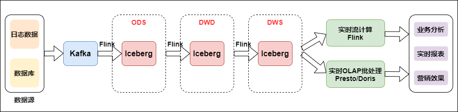
Data is collected from logs to message queues, and then to real-time data warehouses. The construction of basic data flow is unified. Then, for the real-time features of log class, the real-time large screen application adopts real-time stream computing. For Binlog business analysis, take real-time OLAP batch processing.
We can see that the combination of stream and batch has changed from Kafka to iceberg. Iceberg is an intermediate layer between the upper computing engine and the lower storage format. We can define it as a "data organization format". The lower storage is still HDFS. So why add an intermediate layer, Is it better to combine convection and batch processing? Iceberg's ACID capability can simplify the design of the whole pipeline, reduce the delay of the whole pipeline, and its modification and deletion ability can effectively reduce the overhead and improve the efficiency. Iceberg can effectively support batch processing of high throughput data scanning and stream computing, and conduct concurrent real-time processing according to partition granularity.
6, Build a real-time data warehouse from 0 to 1 based on Flink SQL
Note: this section comes from the official account of big data technology and several positions.
Real time data warehouse mainly solves the problem of low data timeliness of traditional data warehouse. Real time data warehouse is usually used for real-time OLAP analysis, real-time large screen display and real-time monitoring and alarm scenes. Although the architecture and technology selection of real-time data warehouse are different from the traditional offline data warehouse, the basic methodology of data warehouse construction is consistent. Next, it mainly introduces the demo of Flink SQL building a real-time data warehouse from 0 to 1, which involves the whole process of data collection, storage, calculation and visualization.
1. Case introduction
Taking e-commerce business as an example, this paper shows the data processing flow of real-time data warehouse. In addition, this paper aims to illustrate the construction process of real-time data warehouse, so it will not involve complex data calculation. In order to ensure the operability and integrity of the case, this paper will give detailed operation steps. For the convenience of demonstration, all operations in this article are completed in Flink SQL Cli.
2. Architecture design
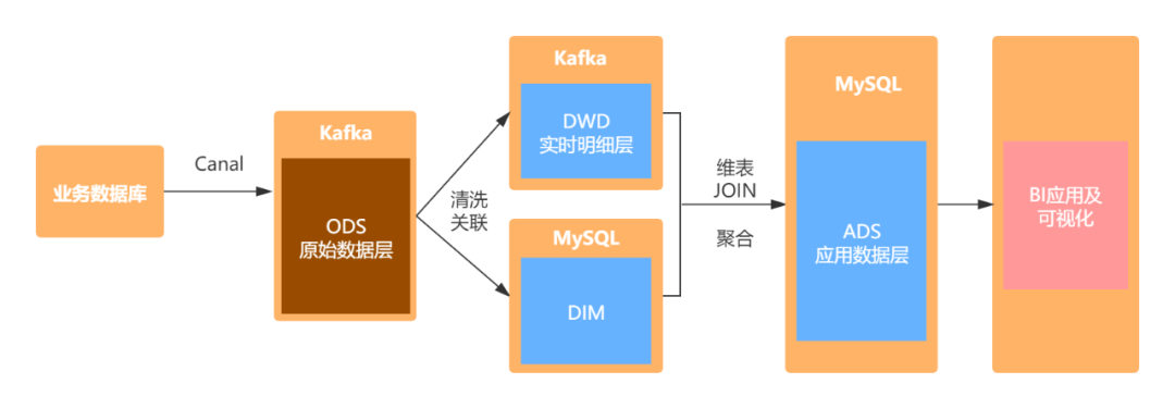
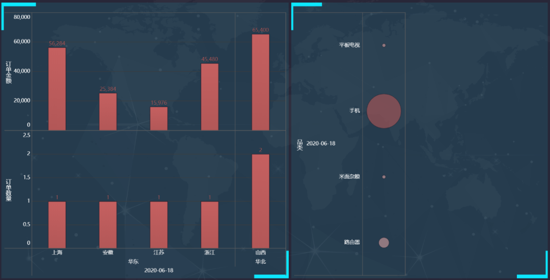
The specific architecture design is shown in the figure: first, parse the binlog log of MySQL through canal and store the data in Kafka. Then, Flink SQL is used to clean and correlate the original data, and the processed schedule is written into Kafka. Dimension table data is stored in mysql, and the detailed wide table and dimension table are join ed through Flink SQL. The aggregated data is written into mysql, and finally visually displayed through FineBI.
3. Business data preparation
1. Order_info
CREATE TABLE `order_info` (
  `id` bigint(20) NOT NULL AUTO_INCREMENT COMMENT 'number',
  `consignee` varchar(100) DEFAULT NULL COMMENT 'consignee',
  `consignee_tel` varchar(20) DEFAULT NULL COMMENT 'Recipient phone',
  `total_amount` decimal(10,2) DEFAULT NULL COMMENT 'Total amount',
  `order_status` varchar(20) DEFAULT NULL COMMENT 'Order status',
  `user_id` bigint(20) DEFAULT NULL COMMENT 'user id',
  `payment_way` varchar(20) DEFAULT NULL COMMENT 'payment method',
  `delivery_address` varchar(1000) DEFAULT NULL COMMENT 'Shipping address',
  `order_comment` varchar(200) DEFAULT NULL COMMENT 'Order remarks',
  `out_trade_no` varchar(50) DEFAULT NULL COMMENT 'Order transaction number (for third party payment))',
  `trade_body` varchar(200) DEFAULT NULL COMMENT 'Order description(For third party payment)',
  `create_time` datetime DEFAULT NULL COMMENT 'Creation time',
  `operate_time` datetime DEFAULT NULL COMMENT 'Operation time',
  `expire_time` datetime DEFAULT NULL COMMENT 'Failure time',
  `tracking_no` varchar(100) DEFAULT NULL COMMENT 'Logistics order No',
  `parent_order_id` bigint(20) DEFAULT NULL COMMENT 'Parent order number',
  `img_url` varchar(200) DEFAULT NULL COMMENT 'Picture path',
  `province_id` int(20) DEFAULT NULL COMMENT 'region',
  PRIMARY KEY (`id`)
) ENGINE=InnoDB AUTO_INCREMENT=1 DEFAULT CHARSET=utf8 COMMENT='Order form';
2. Order_detail
CREATE TABLE `order_detail` (
  `id` bigint(20) NOT NULL AUTO_INCREMENT COMMENT 'number',
  `order_id` bigint(20) DEFAULT NULL COMMENT 'Order number',
  `sku_id` bigint(20) DEFAULT NULL COMMENT 'sku_id',
  `sku_name` varchar(200) DEFAULT NULL COMMENT 'sku Name (redundant))',
  `img_url` varchar(200) DEFAULT NULL COMMENT 'Picture name (redundant))',
  `order_price` decimal(10,2) DEFAULT NULL COMMENT 'Purchase price(When placing an order sku Price)',
  `sku_num` varchar(200) DEFAULT NULL COMMENT 'Number of purchases',
  `create_time` datetime DEFAULT NULL COMMENT 'Creation time',
  PRIMARY KEY (`id`)
) ENGINE=InnoDB AUTO_INCREMENT=1 DEFAULT CHARSET=utf8 COMMENT='Order details';
3. Commodity list (sku_info)
CREATE TABLE `sku_info` (
  `id` bigint(20) NOT NULL AUTO_INCREMENT COMMENT 'skuid(itemID)',
  `spu_id` bigint(20) DEFAULT NULL COMMENT 'spuid',
  `price` decimal(10,0) DEFAULT NULL COMMENT 'Price',
  `sku_name` varchar(200) DEFAULT NULL COMMENT 'sku name',
  `sku_desc` varchar(2000) DEFAULT NULL COMMENT 'Product specification description',
  `weight` decimal(10,2) DEFAULT NULL COMMENT 'weight',
  `tm_id` bigint(20) DEFAULT NULL COMMENT 'brand(redundancy)',
  `category3_id` bigint(20) DEFAULT NULL COMMENT 'Three level classification id(redundancy)',
  `sku_default_img` varchar(200) DEFAULT NULL COMMENT 'Default display picture(redundancy)',
  `create_time` datetime DEFAULT NULL COMMENT 'Creation time',
  PRIMARY KEY (`id`)
) ENGINE=InnoDB AUTO_INCREMENT=1 DEFAULT CHARSET=utf8 COMMENT='Commodity list';
4. Base_category 1
CREATE TABLE `base_category1` (
  `id` bigint(20) NOT NULL AUTO_INCREMENT COMMENT 'number',
  `name` varchar(10) NOT NULL COMMENT 'Classification name',
  PRIMARY KEY (`id`)
) ENGINE=InnoDB AUTO_INCREMENT=1 DEFAULT CHARSET=utf8 COMMENT='Primary classification table';
5. Base_category 2
CREATE TABLE `base_category2` (
  `id` bigint(20) NOT NULL AUTO_INCREMENT COMMENT 'number',
  `name` varchar(200) NOT NULL COMMENT 'Secondary classification name',
  `category1_id` bigint(20) DEFAULT NULL COMMENT 'Primary classification number',
  PRIMARY KEY (`id`)
) ENGINE=InnoDB AUTO_INCREMENT=1 DEFAULT CHARSET=utf8 COMMENT='Secondary classification table';
6. Base_category 3
CREATE TABLE `base_category3` (
  `id` bigint(20) NOT NULL AUTO_INCREMENT COMMENT 'number',
  `name` varchar(200) NOT NULL COMMENT 'Three level classification name',
  `category2_id` bigint(20) DEFAULT NULL COMMENT 'Secondary classification number',
  PRIMARY KEY (`id`)
) ENGINE=InnoDB AUTO_INCREMENT=1 DEFAULT CHARSET=utf8 COMMENT='Three level classification table';
7. base_region_ province)
CREATE TABLE `base_province` (
  `id` int(20) DEFAULT NULL COMMENT 'id',
  `name` varchar(20) DEFAULT NULL COMMENT 'Province name',
  `region_id` int(20) DEFAULT NULL COMMENT 'Large area id',
  `area_code` varchar(20) DEFAULT NULL COMMENT 'Administrative location code'
) ENGINE=InnoDB DEFAULT CHARSET=utf8;
8. Base_region
CREATE TABLE `base_region` (
  `id` int(20) NOT NULL COMMENT 'Large area id',
  `region_name` varchar(20) DEFAULT NULL COMMENT 'Region name',
   PRIMARY KEY (`id`)
) ENGINE=InnoDB DEFAULT CHARSET=utf8;
4. Data processing flow
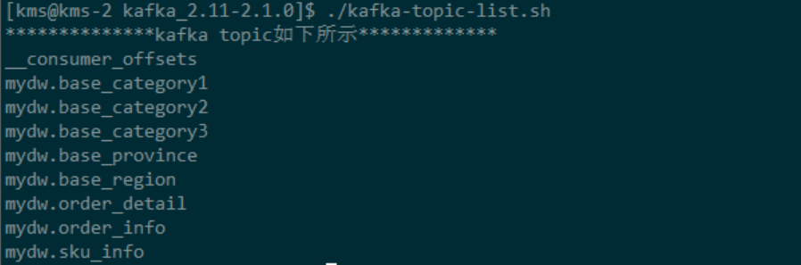
1. ods layer data synchronization
The data synchronization of ODS layer will not be expanded in detail here. It mainly uses canal to parse the binlog log of MySQL, and then writes it to the topic corresponding to Kafka. Due to space constraints, specific details will not be explained. The results after synchronization are shown in the following figure:
2. DIM layer data preparation
In this case, the dimension table is stored in MySQL, and HBase will be used to store dimension table data in actual production. We mainly use two dimension tables: regional dimension table and commodity dimension table. The process is as follows:
- Regional dimension table
First, mydw base_ Province and mydw base_ The data corresponding to the topic of region is extracted into mysql, mainly using the canal JSON format corresponding to the Kafka data source of Flink SQL. Note: before loading, you need to create the corresponding table in MySQL. The name of the MySQL database used in this paper is dim, which is used to store dimension table data. As follows:
-- -------------------------
--   province
--   kafka Source
-- -------------------------
DROP TABLE IF EXISTS `ods_base_province`;
CREATE TABLE `ods_base_province` (
  `id` INT,
  `name` STRING,
  `region_id` INT ,
  `area_code`STRING
) WITH(
'connector' = 'kafka',
 'topic' = 'mydw.base_province',
 'properties.bootstrap.servers' = 'kms-3:9092',
 'properties.group.id' = 'testGroup',
 'format' = 'canal-json' ,
 'scan.startup.mode' = 'earliest-offset'
) ;

-- -------------------------
--   province
--   MySQL Sink
-- -------------------------
DROP TABLE IF EXISTS `base_province`;
CREATE TABLE `base_province` (
    `id` INT,
    `name` STRING,
    `region_id` INT ,
    `area_code`STRING,
    PRIMARY KEY (id) NOT ENFORCED
) WITH (
    'connector' = 'jdbc',
    'url' = 'jdbc:mysql://kms-1:3306/dim',
    'table-name' = 'base_province', -- MySQL Table in which data is to be inserted
    'driver' = 'com.mysql.jdbc.Driver',
    'username' = 'root',
    'password' = '123qwe',
    'sink.buffer-flush.interval' = '1s'
);

-- -------------------------
--   province
--   MySQL Sink Load Data
-- -------------------------
INSERT INTO base_province
SELECT *
FROM ods_base_province;

-- -------------------------
--   region
--   kafka Source
-- -------------------------
DROP TABLE IF EXISTS `ods_base_region`;
CREATE TABLE `ods_base_region` (
  `id` INT,
  `region_name` STRING
) WITH(
'connector' = 'kafka',
 'topic' = 'mydw.base_region',
 'properties.bootstrap.servers' = 'kms-3:9092',
 'properties.group.id' = 'testGroup',
 'format' = 'canal-json' ,
 'scan.startup.mode' = 'earliest-offset'
) ;

-- -------------------------
--   region
--   MySQL Sink
-- -------------------------
DROP TABLE IF EXISTS `base_region`;
CREATE TABLE `base_region` (
    `id` INT,
    `region_name` STRING,
     PRIMARY KEY (id) NOT ENFORCED
) WITH (
    'connector' = 'jdbc',
    'url' = 'jdbc:mysql://kms-1:3306/dim',
    'table-name' = 'base_region', -- MySQL Table in which data is to be inserted
    'driver' = 'com.mysql.jdbc.Driver',
    'username' = 'root',
    'password' = '123qwe',
    'sink.buffer-flush.interval' = '1s'
);

-- -------------------------
--   region
--   MySQL Sink Load Data
-- -------------------------
INSERT INTO base_region
SELECT *
FROM ods_base_region;
After the above steps, the original data required to create a dimension table has been stored in MySQL. Next, we need to create a dimension table in MySQL. We use the above two tables to create a view: dim_province as dimension table:
-- ---------------------------------
-- DIM layer,Regional dimension table,
-- stay MySQL Create view in
-- ---------------------------------
DROP VIEW IF EXISTS dim_province;
CREATE VIEW dim_province AS
SELECT
  bp.id AS province_id,
  bp.name AS province_name,
  br.id AS region_id,
  br.region_name AS region_name,
  bp.area_code AS area_code
FROM base_region br
     JOIN base_province bp ON br.id= bp.region_id;
In this way, we need the dimension table: dim_province is created. You only need to use Flink SQL to create a JDBC data source when join ing the dimension table, and then you can use the dimension table. Similarly, we use the same method to create a commodity dimension table, as follows:
-- -------------------------
--  List of primary categories
--   kafka Source
-- -------------------------
DROP TABLE IF EXISTS `ods_base_category1`;
CREATE TABLE `ods_base_category1` (
  `id` BIGINT,
  `name` STRING
)WITH(
 'connector' = 'kafka',
 'topic' = 'mydw.base_category1',
 'properties.bootstrap.servers' = 'kms-3:9092',
 'properties.group.id' = 'testGroup',
 'format' = 'canal-json' ,
 'scan.startup.mode' = 'earliest-offset'
) ;

-- -------------------------
--  List of primary categories
--   MySQL Sink
-- -------------------------
DROP TABLE IF EXISTS `base_category1`;
CREATE TABLE `base_category1` (
    `id` BIGINT,
    `name` STRING,
     PRIMARY KEY (id) NOT ENFORCED
) WITH (
    'connector' = 'jdbc',
    'url' = 'jdbc:mysql://kms-1:3306/dim',
    'table-name' = 'base_category1', -- MySQL Table in which data is to be inserted
    'driver' = 'com.mysql.jdbc.Driver',
    'username' = 'root',
    'password' = '123qwe',
    'sink.buffer-flush.interval' = '1s'
);

-- -------------------------
--  List of primary categories
--   MySQL Sink Load Data
-- -------------------------

INSERT INTO base_category1
SELECT *
FROM ods_base_category1;

-- -------------------------
--  Secondary category table
--   kafka Source
-- -------------------------
DROP TABLE IF EXISTS `ods_base_category2`;
CREATE TABLE `ods_base_category2` (
  `id` BIGINT,
  `name` STRING,
  `category1_id` BIGINT
)WITH(
'connector' = 'kafka',
 'topic' = 'mydw.base_category2',
 'properties.bootstrap.servers' = 'kms-3:9092',
 'properties.group.id' = 'testGroup',
 'format' = 'canal-json' ,
 'scan.startup.mode' = 'earliest-offset'
) ;

-- -------------------------
--  Secondary category table
--   MySQL Sink
-- -------------------------
DROP TABLE IF EXISTS `base_category2`;
CREATE TABLE `base_category2` (
    `id` BIGINT,
    `name` STRING,
    `category1_id` BIGINT,
     PRIMARY KEY (id) NOT ENFORCED
) WITH (
    'connector' = 'jdbc',
    'url' = 'jdbc:mysql://kms-1:3306/dim',
    'table-name' = 'base_category2', -- MySQL Table in which data is to be inserted
    'driver' = 'com.mysql.jdbc.Driver',
    'username' = 'root',
    'password' = '123qwe',
    'sink.buffer-flush.interval' = '1s'
);

-- -------------------------
--  Secondary category table
--   MySQL Sink Load Data
-- -------------------------
INSERT INTO base_category2
SELECT *
FROM ods_base_category2;

-- -------------------------
-- Class III category table
--   kafka Source
-- -------------------------
DROP TABLE IF EXISTS `ods_base_category3`;
CREATE TABLE `ods_base_category3` (
  `id` BIGINT,
  `name` STRING,
  `category2_id` BIGINT
)WITH(
'connector' = 'kafka',
 'topic' = 'mydw.base_category3',
 'properties.bootstrap.servers' = 'kms-3:9092',
 'properties.group.id' = 'testGroup',
 'format' = 'canal-json' ,
 'scan.startup.mode' = 'earliest-offset'
) ;

-- -------------------------
--  Class III category table
--   MySQL Sink
-- -------------------------
DROP TABLE IF EXISTS `base_category3`;
CREATE TABLE `base_category3` (
    `id` BIGINT,
    `name` STRING,
    `category2_id` BIGINT,
    PRIMARY KEY (id) NOT ENFORCED
) WITH (
    'connector' = 'jdbc',
    'url' = 'jdbc:mysql://kms-1:3306/dim',
    'table-name' = 'base_category3', -- MySQL Table in which data is to be inserted
    'driver' = 'com.mysql.jdbc.Driver',
    'username' = 'root',
    'password' = '123qwe',
    'sink.buffer-flush.interval' = '1s'
);

-- -------------------------
--  Class III category table
--   MySQL Sink Load Data
-- -------------------------
INSERT INTO base_category3
SELECT *
FROM ods_base_category3;

-- -------------------------
--   Commodity list
--   Kafka Source
-- -------------------------

DROP TABLE IF EXISTS `ods_sku_info`;
CREATE TABLE `ods_sku_info` (
  `id` BIGINT,
  `spu_id` BIGINT,
  `price` DECIMAL(10,0),
  `sku_name` STRING,
  `sku_desc` STRING,
  `weight` DECIMAL(10,2),
  `tm_id` BIGINT,
  `category3_id` BIGINT,
  `sku_default_img` STRING,
  `create_time` TIMESTAMP(0)
) WITH(
 'connector' = 'kafka',
 'topic' = 'mydw.sku_info',
 'properties.bootstrap.servers' = 'kms-3:9092',
 'properties.group.id' = 'testGroup',
 'format' = 'canal-json' ,
 'scan.startup.mode' = 'earliest-offset'
) ;

-- -------------------------
--   Commodity list
--   MySQL Sink
-- -------------------------
DROP TABLE IF EXISTS `sku_info`;
CREATE TABLE `sku_info` (
  `id` BIGINT,
  `spu_id` BIGINT,
  `price` DECIMAL(10,0),
  `sku_name` STRING,
  `sku_desc` STRING,
  `weight` DECIMAL(10,2),
  `tm_id` BIGINT,
  `category3_id` BIGINT,
  `sku_default_img` STRING,
  `create_time` TIMESTAMP(0),
   PRIMARY KEY (tm_id) NOT ENFORCED
) WITH (
    'connector' = 'jdbc',
    'url' = 'jdbc:mysql://kms-1:3306/dim',
    'table-name' = 'sku_info', -- MySQL Table in which data is to be inserted
    'driver' = 'com.mysql.jdbc.Driver',
    'username' = 'root',
    'password' = '123qwe',
    'sink.buffer-flush.interval' = '1s'
);

-- -------------------------
--   commodity
--   MySQL Sink Load Data
-- -------------------------
INSERT INTO sku_info
SELECT *
FROM ods_sku_info;
After the above steps, we can synchronize the basic data table of creating commodity dimension table to MySQL. Similarly, we need to create the corresponding data table in advance. Next, we use the above basic table to create a view in the dim Library of MySQL: dim_sku_info, used as a dimension table for subsequent use.
-- ---------------------------------
-- DIM layer,Commodity dimension table,
-- stay MySQL Create view in
-- ---------------------------------
CREATE VIEW dim_sku_info AS
SELECT
  si.id AS id,
  si.sku_name AS sku_name,
  si.category3_id AS c3_id,
  si.weight AS weight,
  si.tm_id AS tm_id,
  si.price AS price,
  si.spu_id AS spu_id,
  c3.name AS c3_name,
  c2.id AS c2_id,
  c2.name AS c2_name,
  c3.id AS c1_id,
  c3.name AS c1_name
FROM
(
  sku_info si
  JOIN base_category3 c3 ON si.category3_id = c3.id
  JOIN base_category2 c2 ON c3.category2_id =c2.id
  JOIN base_category1 c1 ON c2.category1_id = c1.id
);
So far, the dimension table data we need is ready. Next, we start to process the data of DWD layer.
3. DWD layer data processing
After the above steps, we have prepared the dimension table for use. Next, we will process the original data of ODS and process it into the schedule of DWD layer. The specific process is as follows:
-- -------------------------
--   Order details
--   Kafka Source
-- -------------------------

DROP TABLE IF EXISTS `ods_order_detail`;
CREATE TABLE `ods_order_detail`(
  `id` BIGINT,
  `order_id` BIGINT,
  `sku_id` BIGINT,
  `sku_name` STRING,
  `img_url` STRING,
  `order_price` DECIMAL(10,2),
  `sku_num` INT,
  `create_time` TIMESTAMP(0)
) WITH(
 'connector' = 'kafka',
 'topic' = 'mydw.order_detail',
 'properties.bootstrap.servers' = 'kms-3:9092',
 'properties.group.id' = 'testGroup',
 'format' = 'canal-json' ,
 'scan.startup.mode' = 'earliest-offset'
) ;

-- -------------------------
--   Order information
--   Kafka Source
-- -------------------------
DROP TABLE IF EXISTS `ods_order_info`;
CREATE TABLE `ods_order_info` (
  `id` BIGINT,
  `consignee` STRING,
  `consignee_tel` STRING,
  `total_amount` DECIMAL(10,2),
  `order_status` STRING,
  `user_id` BIGINT,
  `payment_way` STRING,
  `delivery_address` STRING,
  `order_comment` STRING,
  `out_trade_no` STRING,
  `trade_body` STRING,
  `create_time` TIMESTAMP(0) ,
  `operate_time` TIMESTAMP(0) ,
  `expire_time` TIMESTAMP(0) ,
  `tracking_no` STRING,
  `parent_order_id` BIGINT,
  `img_url` STRING,
  `province_id` INT
) WITH(
'connector' = 'kafka',
 'topic' = 'mydw.order_info',
 'properties.bootstrap.servers' = 'kms-3:9092',
 'properties.group.id' = 'testGroup',
 'format' = 'canal-json' ,
 'scan.startup.mode' = 'earliest-offset'
) ;

-- ---------------------------------
-- DWD layer,Payment order details dwd_paid_order_detail
-- ---------------------------------
DROP TABLE IF EXISTS dwd_paid_order_detail;
CREATE TABLE dwd_paid_order_detail
(
  detail_id BIGINT,
  order_id BIGINT,
  user_id BIGINT,
  province_id INT,
  sku_id BIGINT,
  sku_name STRING,
  sku_num INT,
  order_price DECIMAL(10,0),
  create_time STRING,
  pay_time STRING
 ) WITH (
    'connector' = 'kafka',
    'topic' = 'dwd_paid_order_detail',
    'scan.startup.mode' = 'earliest-offset',
    'properties.bootstrap.servers' = 'kms-3:9092',
    'format' = 'changelog-json'
);
-- ---------------------------------
-- DWD layer,Paid order details
-- towards dwd_paid_order_detail Load data
-- ---------------------------------
INSERT INTO dwd_paid_order_detail
SELECT
  od.id,
  oi.id order_id,
  oi.user_id,
  oi.province_id,
  od.sku_id,
  od.sku_name,
  od.sku_num,
  od.order_price,
  oi.create_time,
  oi.operate_time
FROM
    (
    SELECT *
    FROM ods_order_info
    WHERE order_status = '2' -- Paid
    ) oi JOIN
    (
    SELECT *
    FROM ods_order_detail
    ) od
    ON oi.id = od.order_id;
4. ADS layer data
After the above steps, we created a dwd_paid_order_detail schedule and stored it in Kafka. Next, we will use this detail wide table and dimension table to JOIN to get our ADS application layer data.
- ads_province_index
First, create the corresponding ADS target table in MySQL: ads_province_index
CREATE TABLE ads.ads_province_index(
  province_id INT(10),
  area_code VARCHAR(100),
  province_name VARCHAR(100),
  region_id INT(10),
  region_name VARCHAR(100),
  order_amount DECIMAL(10,2),
  order_count BIGINT(10),
  dt VARCHAR(100),
  PRIMARY KEY (province_id, dt)
) ;
Load data to the ADS layer target of MySQL:
-- Flink SQL Cli operation
-- ---------------------------------
-- use DDL establish MySQL Medium ADS Layer table
-- Indicator: 1.Orders per province per day
-- 2.Amount of each order per day per Province
-- ---------------------------------
CREATE TABLE ads_province_index(
province_id INT,
area_code STRING,
province_name STRING,
region_id INT,
region_name STRING,
order_amount DECIMAL(10,2),
order_count BIGINT,
dt STRING,
PRIMARY KEY (province_id, dt) NOT ENFORCED
) WITH (
'connector' = 'jdbc',
'url' = 'jdbc:mysql://kms-1:3306/ads',
'table-name' = 'ads_province_index',
'driver' = 'com.mysql.jdbc.Driver',
'username' = 'root',
'password' = '123qwe'
);
-- ---------------------------------
-- dwd_paid_order_detail Paid order details
-- ---------------------------------
CREATE TABLE dwd_paid_order_detail
(
detail_id BIGINT,
order_id BIGINT,
user_id BIGINT,
province_id INT,
sku_id BIGINT,
sku_name STRING,
sku_num INT,
order_price DECIMAL(10,2),
create_time STRING,
pay_time STRING
) WITH (
'connector' = 'kafka',
'topic' = 'dwd_paid_order_detail',
'scan.startup.mode' = 'earliest-offset',
'properties.bootstrap.servers' = 'kms-3:9092',
'format' = 'changelog-json'
);
-- ---------------------------------
-- tmp_province_index
-- Order summary temporary table
-- ---------------------------------
CREATE TABLE tmp_province_index(
province_id INT,
order_count BIGINT,-- Number of orders
order_amount DECIMAL(10,2), -- Order amount
pay_date DATE
)WITH (
'connector' = 'kafka',
'topic' = 'tmp_province_index',
'scan.startup.mode' = 'earliest-offset',
'properties.bootstrap.servers' = 'kms-3:9092',
'format' = 'changelog-json'
);
-- ---------------------------------
-- tmp_province_index
-- Loading order summary temporary table data
-- ---------------------------------
INSERT INTO tmp_province_index
SELECT
province_id,
count(distinct order_id) order_count,-- Number of orders
sum(order_price * sku_num) order_amount, -- Order amount
TO_DATE(pay_time,'yyyy-MM-dd') pay_date
FROM dwd_paid_order_detail
GROUP BY province_id,TO_DATE(pay_time,'yyyy-MM-dd')
;
-- ---------------------------------
-- tmp_province_index_source
-- Use this temporary summary table as the data source
-- ---------------------------------
CREATE TABLE tmp_province_index_source(
province_id INT,
order_count BIGINT,-- Number of orders
order_amount DECIMAL(10,2), -- Order amount
pay_date DATE,
proctime as PROCTIME() -- A processing time column is generated by calculating the column
) WITH (
'connector' = 'kafka',
'topic' = 'tmp_province_index',
'scan.startup.mode' = 'earliest-offset',
'properties.bootstrap.servers' = 'kms-3:9092',
'format' = 'changelog-json'
);
-- ---------------------------------
-- DIM layer,Regional dimension table,
-- Create area dimension table data source
-- ---------------------------------
DROP TABLE IF EXISTS `dim_province`;
CREATE TABLE dim_province (
province_id INT,
province_name STRING,
area_code STRING,
region_id INT,
region_name STRING ,
PRIMARY KEY (province_id) NOT ENFORCED
) WITH (
'connector' = 'jdbc',
'url' = 'jdbc:mysql://kms-1:3306/dim',
'table-name' = 'dim_province',
'driver' = 'com.mysql.jdbc.Driver',
'username' = 'root',
'password' = '123qwe',
'scan.fetch-size' = '100'
);
-- ---------------------------------
-- towards ads_province_index Load data
-- Dimension table JOIN
-- ---------------------------------
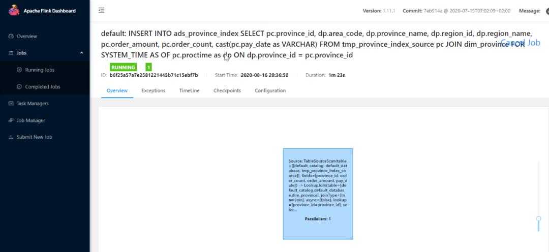
INSERT INTO ads_province_index
SELECT
pc.province_id,
dp.area_code,
dp.province_name,
dp.region_id,
dp.region_name,
pc.order_amount,
pc.order_count,
cast(pc.pay_date as VARCHAR)
FROM
tmp_province_index_source pc
JOIN dim_province FOR SYSTEM_TIME AS OF pc.proctime as dp
ON dp.province_id = pc.province_id;
After submitting the task: observe the Flink WEB UI:
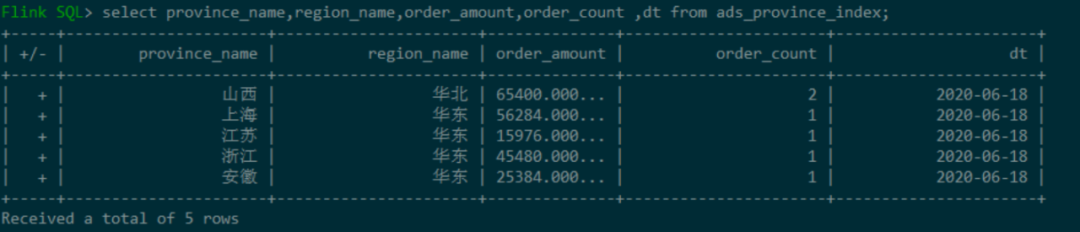
View ADS of ADS layer_ province_ Index table data:
- ads_sku_index
First, create the corresponding ADS target table in MySQL: ads_sku_index
CREATE TABLE ads_sku_index
(
  sku_id BIGINT(10),
  sku_name VARCHAR(100),
  weight DOUBLE,
  tm_id BIGINT(10),
  price DOUBLE,
  spu_id BIGINT(10),
  c3_id BIGINT(10),
  c3_name VARCHAR(100) ,
  c2_id BIGINT(10),
  c2_name VARCHAR(100),
  c1_id BIGINT(10),
  c1_name VARCHAR(100),
  order_amount DOUBLE,
  order_count BIGINT(10),
  sku_count BIGINT(10),
  dt varchar(100),
  PRIMARY KEY (sku_id,dt)
);
Load data to the ADS layer target of MySQL:
-- ---------------------------------
-- use DDL establish MySQL Medium ADS Layer table
-- Indicator: 1.Number of orders corresponding to each commodity per day
-- 2.Order amount corresponding to each commodity every day
-- 3.Quantity of each item per day
-- ---------------------------------
CREATE TABLE ads_sku_index
(
sku_id BIGINT,
sku_name VARCHAR,
weight DOUBLE,
tm_id BIGINT,
price DOUBLE,
spu_id BIGINT,
c3_id BIGINT,
c3_name VARCHAR ,
c2_id BIGINT,
c2_name VARCHAR,
c1_id BIGINT,
c1_name VARCHAR,
order_amount DOUBLE,
order_count BIGINT,
sku_count BIGINT,
dt varchar,
PRIMARY KEY (sku_id,dt) NOT ENFORCED
) WITH (
'connector' = 'jdbc',
'url' = 'jdbc:mysql://kms-1:3306/ads',
'table-name' = 'ads_sku_index',
'driver' = 'com.mysql.jdbc.Driver',
'username' = 'root',
'password' = '123qwe'
);
-- ---------------------------------
-- dwd_paid_order_detail Paid order details
-- ---------------------------------
CREATE TABLE dwd_paid_order_detail
(
detail_id BIGINT,
order_id BIGINT,
user_id BIGINT,
province_id INT,
sku_id BIGINT,
sku_name STRING,
sku_num INT,
order_price DECIMAL(10,2),
create_time STRING,
pay_time STRING
) WITH (
'connector' = 'kafka',
'topic' = 'dwd_paid_order_detail',
'scan.startup.mode' = 'earliest-offset',
'properties.bootstrap.servers' = 'kms-3:9092',
'format' = 'changelog-json'
);
-- ---------------------------------
-- tmp_sku_index
-- Commodity index statistics
-- ---------------------------------
CREATE TABLE tmp_sku_index(
sku_id BIGINT,
order_count BIGINT,-- Number of orders
order_amount DECIMAL(10,2), -- Order amount
order_sku_num BIGINT,
pay_date DATE
)WITH (
'connector' = 'kafka',
'topic' = 'tmp_sku_index',
'scan.startup.mode' = 'earliest-offset',
'properties.bootstrap.servers' = 'kms-3:9092',
'format' = 'changelog-json'
);
-- ---------------------------------
-- tmp_sku_index
-- Data loading
-- ---------------------------------
INSERT INTO tmp_sku_index
SELECT
sku_id,
count(distinct order_id) order_count,-- Number of orders
sum(order_price * sku_num) order_amount, -- Order amount
sum(sku_num) order_sku_num,
TO_DATE(pay_time,'yyyy-MM-dd') pay_date
FROM dwd_paid_order_detail
GROUP BY sku_id,TO_DATE(pay_time,'yyyy-MM-dd')
;
-- ---------------------------------
-- tmp_sku_index_source
-- Use this temporary summary table as the data source
-- ---------------------------------
CREATE TABLE tmp_sku_index_source(
sku_id BIGINT,
order_count BIGINT,-- Number of orders
order_amount DECIMAL(10,2), -- Order amount
order_sku_num BIGINT,
pay_date DATE,
proctime as PROCTIME() -- A processing time column is generated by calculating the column
) WITH (
'connector' = 'kafka',
'topic' = 'tmp_sku_index',
'scan.startup.mode' = 'earliest-offset',
'properties.bootstrap.servers' = 'kms-3:9092',
'format' = 'changelog-json'
);
-- ---------------------------------
-- DIM layer,Commodity dimension table,
-- Create commodity dimension table data source
-- ---------------------------------
DROP TABLE IF EXISTS `dim_sku_info`;
CREATE TABLE dim_sku_info (
id BIGINT,
sku_name STRING,
c3_id BIGINT,
weight DECIMAL(10,2),
tm_id BIGINT,
price DECIMAL(10,2),
spu_id BIGINT,
c3_name STRING,
c2_id BIGINT,
c2_name STRING,
c1_id BIGINT,
c1_name STRING,
PRIMARY KEY (id) NOT ENFORCED
) WITH (
'connector' = 'jdbc',
'url' = 'jdbc:mysql://kms-1:3306/dim',
'table-name' = 'dim_sku_info',
'driver' = 'com.mysql.jdbc.Driver',
'username' = 'root',
'password' = '123qwe',
'scan.fetch-size' = '100'
);
-- ---------------------------------
-- towards ads_sku_index Load data
-- Dimension table JOIN
-- ---------------------------------
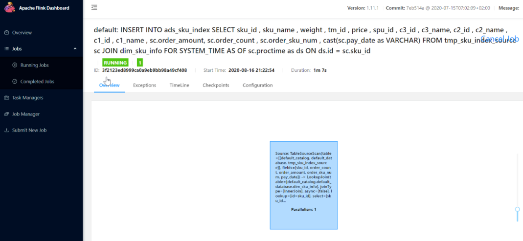
INSERT INTO ads_sku_index
SELECT
sku_id ,
sku_name ,
weight ,
tm_id ,
price ,
spu_id ,
c3_id ,
c3_name,
c2_id ,
c2_name ,
c1_id ,
c1_name ,
sc.order_amount,
sc.order_count ,
sc.order_sku_num ,
cast(sc.pay_date as VARCHAR)
FROM
tmp_sku_index_source sc
JOIN dim_sku_info FOR SYSTEM_TIME AS OF sc.proctime as ds
ON ds.id = sc.sku_id;
After submitting the task: observe the Flink WEB UI:
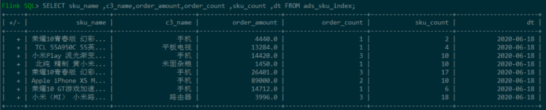
View ADS of ADS layer_ sku_ Index table data:
5. FineBI display
7, Data governance
The real difficulty of data warehouse construction lies not in the design of data warehouse, but in the data governance after the subsequent business develops and the business line becomes huge, including asset governance, data quality monitoring, data index system construction, etc.
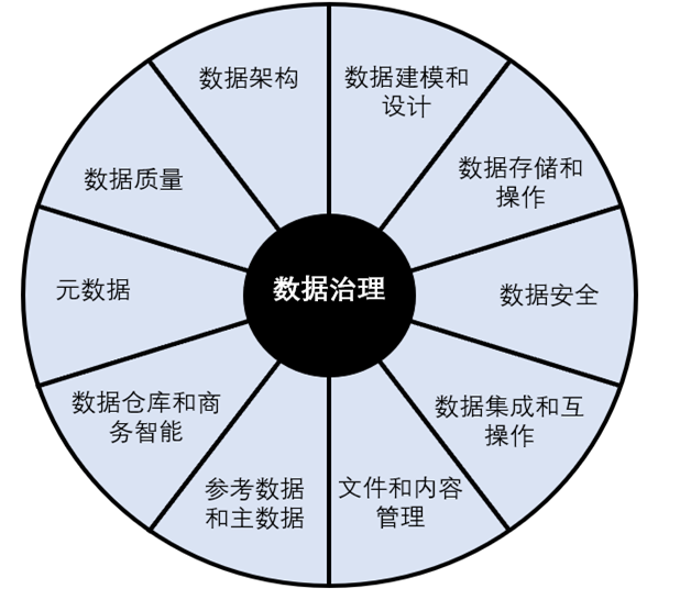
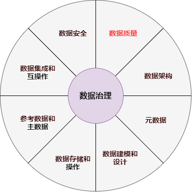
In fact, the scope of data governance is very wide, including data book management, data security, data quality, data cost, etc. In the DAMA data management knowledge system guide, data governance is located in the center of the "wheel chart" of data management. It is the general outline of 10 data management fields, such as data architecture, data modeling, data storage, data security, data quality, metadata management and master data management, and provides overall guidance strategies for various data management activities.
1. What is the way of data governance
1. Data governance needs system construction
In order to give full play to the value of data, we need to meet three elements: reasonable platform architecture, perfect governance services and systematic operation means.
Select the appropriate platform architecture according to the scale, industry and data volume of the enterprise; Governance services need to run through the whole life cycle of data to ensure the integrity, accuracy, consistency and effectiveness of data in the whole process of collection, processing, sharing, storage and application; The operation means should include the optimization of norms, organization, platform and process.
2. Data governance needs to lay a solid foundation
Data governance needs to be gradual, but at least three aspects need to be paid attention to in the early stage of Construction: data specification, data quality and data security. Standardized model management is a prerequisite for ensuring that data can be managed, high-quality data is a prerequisite for data availability, and data security control is a prerequisite for data sharing and exchange.
3. Data governance requires IT empowerment
Data governance is not a pile of normative documents, but the norms, processes and standards generated in the governance process need to be implemented on the IT platform. In the process of data production, data governance is carried out in a forward way of "starting from the end", so as to avoid all kinds of passivity and increase of operation and maintenance costs caused by post audit.
4. Data governance needs to focus on data
The essence of data governance is to manage data. Therefore, it is necessary to strengthen metadata management and master data management, manage data from the source, supplement relevant attributes and information of data, such as metadata, quality, safety, business logic, blood relationship, etc., and manage data production, processing and use in a metadata driven manner.
5. Data governance requires the integration of construction and management
The consistency between blood relationship of data model and task scheduling is the key to the integration of construction and management, which helps to solve the problem of inconsistency between data management and data production, and avoid the inefficient management mode of two skins.
2. Talking about data governance
As mentioned above, the scope of data governance is very wide, among which the most important is data quality governance, and the scope of data quality is also very wide. It runs through the whole life cycle of data warehouse, from data generation - > data access - > data storage - > Data Processing - > data output - > data display. Quality governance is required in each stage, and the evaluation dimensions include integrity, standardization, consistency Accuracy, uniqueness, relevance, etc.
In each stage of system construction, data quality detection and standardization should be carried out according to the standards, and governance should be carried out in time to avoid post cleaning.
Quality inspection can refer to the following dimensions:
| dimension | Measurement standard |
|---|---|
| Integrity | Whether the necessary data specified by the business is missing, and it is not allowed to be null characters or null values. For example, whether the data source is complete, whether the dimension value is complete, and whether the data value is complete |
| Timeliness | Whether the data can reflect the current facts when needed. That is, the data must be timely and can meet the requirements of the system for data time. For example, timeliness of processing (acquisition, sorting, cleaning, loading, etc.) |
| Uniqueness | Is the data value unique in the specified dataset |
| Referential integrity | Is the data item defined in the parent table |
| Dependency consistency | Whether the data item value satisfies the dependency with other data items |
| Correctness | Whether the data content and definition are consistent |
| Accuracy | Does the data accuracy meet the number of digits required by business rules |
| Technical effectiveness | Are data items organized according to defined format standards |
| Business effectiveness | Whether the data item conforms to the defined |
| reliability | Obtained according to customer survey or customer initiative |
| usability | The ratio of the time data is available to the time data needs to be accessed |
| Accessibility | Is the data easy to read automatically |
Here are some specific governance methods summarized according to meituan's technical articles:
1. Standardize governance
Standardization is the guarantee of data warehouse construction. In order to avoid repeated construction of indicators and poor data quality, standardized construction shall be carried out in accordance with the most detailed and landing method.
(1) Root word
Root is the basis of dimension and index management. It is divided into common root and proprietary root to improve the ease of use and relevance of root.
-
Common root: the smallest unit describing things, such as transaction trade.
-
Proper word root: it has a conventional or industry-specific description, such as USD USD.
(2) Table naming conventions
General specification
-
Table names and field names are separated by an underscore (example: clienttype - > client_type).
-
Each part uses lowercase English words. If it belongs to general field, it must meet the definition of general field information.
-
Table name and field name must start with a letter.
-
The maximum length of table name and field name shall not exceed 64 English characters.
-
Give priority to the existing keywords in the root (root management in the standard configuration of data warehouse), and regularly Review the irrationality of new naming.
-
Non standard abbreviations are prohibited in the table name customization part.
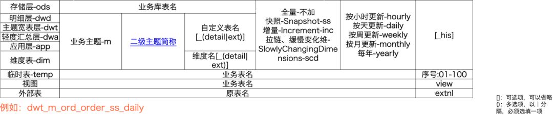
Table naming rules
- Table name = type + business topic + sub topic + table meaning + storage format + update frequency + end, as shown in the following figure:
(3) Index naming specification
Combined with the characteristics of the index and the specification of word root management, the index is structured.
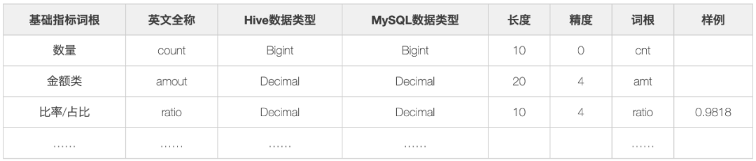
- Basic indicator root, that is, all indicators must contain the following basic root:
- Business modifiers are words used to describe business scenarios, such as trade transaction.
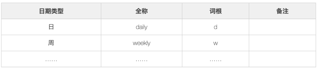
3. Date modifier, used to modify the time interval of business occurrence.
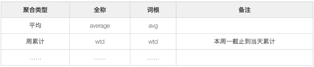
4. Aggregate modifier to aggregate the results.
5. Basic indicator: a single business modifier + basic indicator root constructs a basic indicator, such as transaction amount trade_amt.
6. Derived indicators: multi modifier + basic indicator root to construct derived indicators. Derived indicators inherit the characteristics of basic indicators, for example: number of installed Stores - install_poi_cnt.
7. The naming standard of common indicators is consistent with the field naming standard, which can be converted by vocabulary. 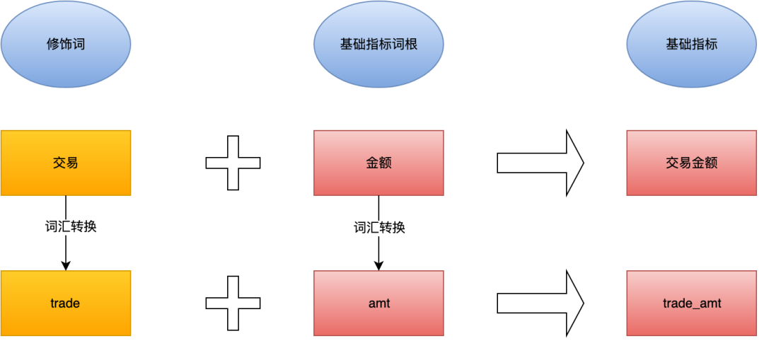
2. Structure governance
(1) Data layering
An excellent and reliable data warehouse system often requires a clear data layered structure, that is, to ensure the stability of the data layer, shield the impact on the downstream, and avoid long links. The general layered structure is as follows: 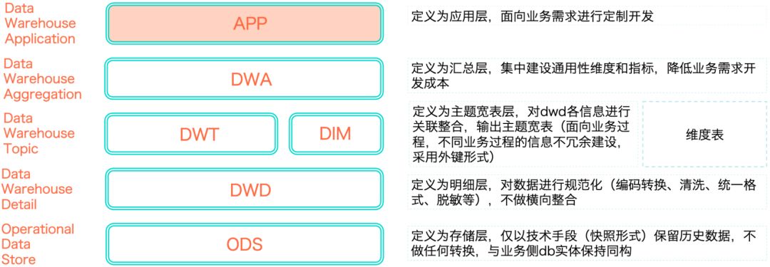
(2) Data flow direction
The stable business is developed according to the standard data flow, that is, ODS -- > DWD -- > DWA -- > app. Unstable business or exploratory requirements can follow the two model data flows of ODS - > DWD - > app or ODS - > DWD - > DWT - > app. After ensuring the rationality of the data link, the layered reference principle of the model is confirmed on this basis:
-
Normal flow direction: ODS > DWD - > DWT - > DWA - > app. When the relationship of ODS > DWD - > DWA - > app appears, it indicates that the subject field is not covered completely. DWD data should be put into DWT. DWD - > DWA is allowed for tables with very low frequency of use.
-
Try to avoid tables that use DWD and DWT (the subject domain to which the DWD belongs) in DWA wide tables.
-
In principle, DWT tables generated by DWT in the same subject domain should be avoided as much as possible, otherwise it will affect the efficiency of ETL.
-
Direct use of ODS tables is prohibited in DWT, DWA and APP. ODS tables can only be referenced by DWD.
-
Reverse dependencies are prohibited. For example, DWT tables depend on DWA tables.
3. Metadata governance
Metadata can be divided into Technical Metadata and business metadata:
Technical metadata is used by IT personnel who develop and manage data warehouse. It describes the data related to the development, management and maintenance of data warehouse, including data source information, data transformation description, data warehouse model, data cleaning and update rules, data mapping and access rights, etc.
Common technical metadata include:
-
Store metadata: such as tables, fields, partitions and other information.
-
Running metadata: such as the running information of all jobs on the big data platform: similar to Hive Job log, including job type, instance name, input and output, SQL, running parameters, execution time, execution engine, etc.
-
Data synchronization, computing tasks, task scheduling and other information in the data development platform: including the input and output tables and fields of data synchronization, as well as the node information of the synchronization task itself: computing tasks mainly include input and output, node information of the task itself, and task scheduling mainly includes the dependency types and dependencies of tasks, as well as the operation logs of different types of scheduling tasks.
-
Data quality and operation and maintenance related metadata: such as task monitoring, operation and maintenance alarm, data quality, fault and other information, including task monitoring operation log, alarm configuration and operation log, fault information, etc.
Business metadata serves the management and business analysts. It describes the data from a business perspective, including business terms, what data is in the data warehouse, the location of the data and the availability of the data, so as to help business personnel better understand what data is available in the data warehouse and how to use it.
- Common business metadata includes standardized definitions of dimensions and attributes (including dimension code, field type, creator, creation time, status, etc.), business process, indicators (including indicator name, indicator code, business caliber, indicator type, person in charge, creation time, status, sql, etc.), security level, calculation logic, etc., which are used to better manage and use data. Data application metadata, such as configuration and operation metadata of data reports, data products, etc.
Metadata not only defines the mode, source, extraction and conversion rules of data in the data warehouse, but also is the basis of the operation of the whole data warehouse system. Metadata connects various loose components in the data warehouse system to form an organic whole.
Metadata governance mainly solves three problems:
-
Promote the implementation of business standards by establishing corresponding organizations, processes and tools, realize the standardized definition of indicators and eliminate the ambiguity of indicator cognition;
-
Based on the current business situation and future evolution mode, abstract the business model, formulate clear themes, business processes and analysis directions, construct complete technical metadata, accurately and perfectly describe the physical model, open up the relationship between Technical Metadata and business metadata, and completely describe the physical model;
-
Through the construction of metadata, improve the efficiency of using data, and solve the problems of "finding, understanding and evaluation" and "data retrieval and data visualization".
4. Security Governance
Around the data security standards, first of all, there should be data classification and classification standards to ensure that the data has an accurate security level before going online. Second, for data users, there should be clear role authorization standards to ensure that important data cannot be taken away through hierarchical classification and role authorization. Third, for sensitive data, there should be privacy management standards to ensure the safe storage of sensitive data. Even if unauthorized users bypass permission management to get sensitive data, they should also ensure that they can't understand it. Fourth, through the development of audit standards, provide audit basis for follow-up audit and ensure that the data can not go away.
5. Data lifecycle governance
Everything has a certain life cycle, and data is no exception. There should be a scientific management method for the generation, processing, use and even extinction of data. Stripping the little or no longer used data from the system and retaining it through the verified storage equipment can not only improve the operation efficiency of the system and better serve customers, but also greatly reduce the storage cost caused by the long-term preservation of data. The data life cycle generally includes three stages: online stage, archiving stage (sometimes further divided into online archiving stage and offline archiving stage) and destruction stage. The management content includes establishing reasonable data categories and formulating retention time, storage medium, cleaning rules and methods, precautions, etc. for different types of data.
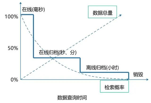
From the relationship between the parameters in the data life cycle in the figure above, we can see that data life cycle management can greatly improve the query efficiency of high-value data, and the purchase of high-priced storage media can also be greatly reduced; However, with the decline in the use of data, the data is gradually archived, and the query time is also slowly getting longer; Finally, as the frequency and value of the data are basically gone, it can be gradually destroyed.
Guess you like:
-
Meituan data platform and data warehouse construction practice, over 100000 words summary
-
Hundreds of high-quality big data books with a required reading list (big data treasure)
-
50000 words | it took a month to sort out this Hadoop blood spitting dictionary
8, Data quality construction
The scope of data governance is very wide, including data book management, data security, data quality, data cost, etc. Among so many governance contents, what is the most important governance? Of course, it is data quality management, because data quality is not only the basis of the effectiveness and accuracy of data analysis conclusions, but also the premise of all this. Therefore, how to ensure data quality and data availability is a link that can not be ignored in the construction of data warehouse.
Data quality also covers a wide range and runs through the whole life cycle of data warehouse. From data generation - > data access - > data storage - > Data Processing - > data output - > data display, quality management is required in each stage.
In each stage of system construction, data quality detection and standardization should be carried out according to the standards, and governance should be carried out in time to avoid post cleaning.
This document is first published in the official account [five minutes learning big data], and the complete data management and warehouse building articles are available on the official account.
1. Why data quality assessment
Many novice data people will immediately start various exploration and statistical analysis of the data after they get the data, in an attempt to immediately find the information and knowledge hidden behind the data. However, after working for a while, I found that I couldn't extract too much valuable information and wasted a lot of time and energy in vain. For example, in the process of dealing with data, the following scenarios may occur:
Scenario 1: as a data analyst, I need to make statistics on the purchase of users in the past 7 days. As a result, I found that many data were recorded repeatedly from the data warehouse, and even some data statistical units were not unified.
Scenario 2: the business looks at the report and finds that the transaction gmv plummeted on a certain day. After investigation, it is found that the data on that day is missing.
An important factor causing this situation is the neglect of the objective evaluation of data quality and the failure to formulate reasonable measurement standards, resulting in the failure to find problems in the data. Therefore, it is very necessary and important to measure the data quality scientifically and objectively.
2. Data quality measurement standard
There are different standards in the industry on how to evaluate the quality of data. I summarize the following six dimensions for evaluation, including integrity, standardization, consistency, accuracy, uniqueness and timeliness.
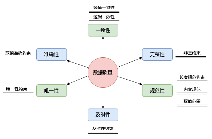
- Data integrity
The possibility of missing information in a field is also the possibility of missing data in the record.
- Data normalization
Normalization refers to the degree to which data follows predetermined syntax rules and whether it conforms to its definition, such as data type, format, value range, etc.
- Data consistency
Consistency refers to whether the data follows a unified specification and whether the data set maintains a unified format. The consistency of data quality is mainly reflected in the specification of data records and whether the data conforms to logic. Consistency does not mean that the values are absolutely the same, but the methods and standards of data collection and processing. Common consistency indicators include: ID coincidence degree, consistent attributes, consistent values, consistent collection methods and consistent transformation steps.
- Data accuracy
Accuracy refers to whether there are abnormalities or errors in the information recorded in the data. Unlike consistency, the data with accuracy problems is not only inconsistent in rules, but also common data accuracy errors, such as garbled code. Secondly, abnormally large or small data are also unqualified data. Common accuracy indicators include: proportion of missing values, proportion of wrong values, proportion of abnormal values, sampling deviation and data noise.
- Data uniqueness
Uniqueness means that there is no duplication of data in the database. For example, there are 10000 real transactions, but there are 3000 duplicates in the data sheet, which has become 13000 transaction records. This data does not meet the data uniqueness.
- Data timeliness
Timeliness refers to the time interval between data generation and viewing, also known as the delay time of data. For example, a piece of data is counted offline today, and the results can only be counted the next day or even the third day. This kind of data does not meet the timeliness of data.
There are other measures, which are briefly listed here:
| dimension | Measurement standard |
|---|---|
| Referential integrity | Is the data item defined in the parent table |
| Dependency consistency | Whether the data item value satisfies the dependency with other data items |
| Correctness | Whether the data content and definition are consistent |
| Accuracy | Does the data accuracy meet the number of digits required by business rules |
| Technical effectiveness | Are data items organized according to defined format standards |
| Business effectiveness | Whether the data item conforms to the defined |
| reliability | Obtained according to customer survey or customer initiative |
| usability | The ratio of the time data is available to the time data needs to be accessed |
| Accessibility | Is the data easy to read automatically |
3. Data quality management process
The process of this section is shown in the figure below:
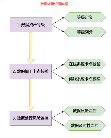
1. Data asset level
1) Level definition
The asset level of data is classified according to the impact on the business when the data quality does not meet the requirements of integrity, standardization, consistency, accuracy, uniqueness and timeliness.
-
Devastating: once the data is wrong, it will cause huge asset losses and face major income damage. Marked L1
-
Global: data is used for group business, enterprise level effect evaluation and important decision-making tasks. Mark as L2
-
Locality: data is used for the daily operation, analysis report, etc. of a business line. If there is a problem, it will have a certain impact on the business line or affect its work efficiency. Marked L3
-
Generality: data is used for daily data analysis, and the impact of problems is very small. Marked as L4
-
Unknown nature: application scenario where data cannot be traced. Marked as Lx
Importance: L1 > L2 > L3 > L4 > LX. If a piece of data appears in multiple application scenarios, it is marked according to its most important degree.
2) Grading
After defining the data asset level, we can mark the data asset level from the data process link, complete the data asset level confirmation, and define different importance levels for different data.
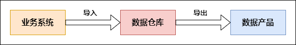
1. Analyze data link:
Data is generated from the business system and enters the data warehouse system through the synchronization tool. After a series of operations in the data warehouse, such as cleaning, processing, integration, algorithm and model in the general sense, it is output to the data products for consumption through the synchronization tool. From the business system to the data warehouse and then to the data products, they are all embodied in the form of tables. The flow process is shown in the figure below:
2. Tag data asset level:
On all data links, sort out the application business of consumption tables. By dividing these application services into data asset levels and combining the upstream and downstream dependencies of data, the whole link is labeled with a certain type of asset level.
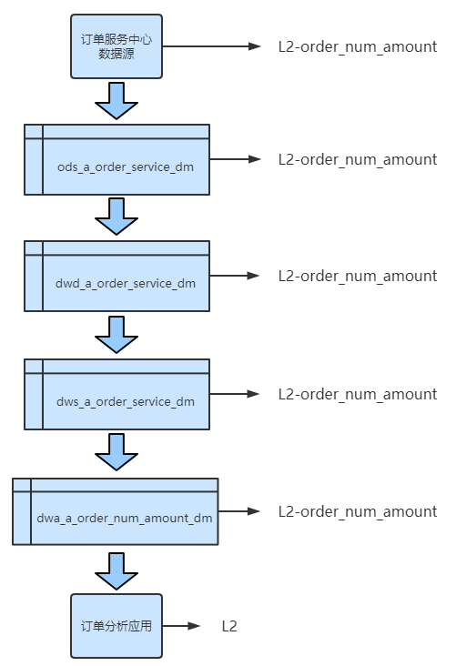
give an example:
Suppose the company has a unified order service center. The application business of the application layer counts the company's order quantity and order amount according to the business line, commodity type and region, and is named order_num_amount.
It is assumed that the data link of the enterprise can be marked as L2-order, which can affect the whole data link of the enterprise_ num_ Amount is marked to the source data business system, as shown in the following figure:
2. Checkpoint verification during data processing
1) Online system data verification
The online business is complex and changeable, and it is always changing. Every change will bring changes to the data. The data warehouse needs to adapt to this changeable business development and achieve the accuracy of the data in time.
Based on this, how to efficiently notify the changes of online business to the offline data warehouse is also a problem to be considered. In order to ensure the consistency of online data and offline data, we can solve the above problems as much as possible through the parallel way of Tool + personnel management: we should not only automatically capture each business change on the tool, but also require developers to automatically notify business change consciously.
1. Business launch platform:
Monitor major business changes on the business online publishing platform, and timely notify the data Department of the changes by subscribing to the publishing process.
As the business system is complex and changeable, if the daily release changes frequently, the data Department will be notified every time, which will cause unnecessary waste of resources. At this time, we can use the previously marked data asset level label to sort out what types of business changes will affect the data processing or the adjustment of data statistical caliber for the data assets involving high-level data applications. These situations must be notified to the data department in time.
If the company does not have its own business publishing platform, it needs to make an agreement with the business department. For business changes of high-level data assets, it needs to be fed back to the data department in time by email or other written instructions.
2. Operator management:
Tools are only a means to assist supervision, and the personnel using tools are the core. The upstream and downstream connection process of data asset level needs to be notified to online business system developers to make them know which are important core data assets and which are only used as internal analysis data for the time being, so as to improve the data risk awareness of online developers.
Through training, online developers can be informed of the demands of data quality management, the whole data processing process of data quality management, as well as the application mode and application scenario of data products, so that they can understand the importance, value and risk of data. Ensure that online developers should consider the goal of data while achieving business goals, and keep the business end and data segment consistent.
2) Offline system data verification
In the process of data from online business system to data warehouse and then to data products, data cleaning and processing need to be completed at the layer of data warehouse. It is the processing of data that leads to the construction of data warehouse model and data warehouse code. How to ensure the quality of data processing is an important link for offline data warehouse to ensure data quality.
In these links, we can adopt the following methods to ensure data quality:
- Code submission verification:
Develop relevant rule engine to assist code submission verification. The rules are roughly classified as follows:
-
Code specification rules: such as table naming specification, field naming specification, life cycle setting, table annotation, etc;
-
Code quality rules: such as the reminder that the denominator is 0, the reminder that NUll value participates in calculation, etc;
-
Code performance rules: such as large table reminder, repeated calculation monitoring, size table join operation reminder, etc.
- Code release verification:
Strengthen the testing link. After the test environment is tested, it is released to the generation environment, and the release is successful only after the generation environment test passes.
- Task change or rerun data:
Before the data update operation, it is necessary to notify the downstream data change reason, change logic, change time and other information. After the downstream has no objection, the change release operation shall be carried out according to the agreed time.
3. Data processing and risk monitoring
Risk point monitoring is mainly to monitor the risks that are easy to occur in the daily operation of data and set up an alarm mechanism, mainly including online data and offline data operation risk point monitoring.
1) Data quality monitoring
The data production process of the online business system needs to ensure the data quality, which is mainly monitored according to the business rules.
For example, some monitoring rules configured in the transaction system, such as order capture time, order completion time, order payment amount, order status flow, etc., are configured with verification rules. The order taking time will certainly not be greater than the time of the day, nor less than the business online time. Once there is an abnormal order creation time, an alarm will be sent immediately to multiple people at the same time. Through this mechanism, problems can be found and solved in time.
With the improvement of business responsibility, there will be many rules and the operation cost of rule configuration will increase. At this time, targeted monitoring can be carried out according to our previous data asset level.
Offline data risk point monitoring mainly includes the monitoring of data accuracy and timeliness of data output. Monitor all data processing scheduling on the data scheduling platform.
We take Alibaba's DataWorks data scheduling tool as an example. DataWorks is a one-stop development workshop based on MaxCompute computing engine to help enterprises quickly complete a full set of data research and development work such as data integration, development, governance, quality and security.
DQC in DataWorks realizes the data quality monitoring and alarm mechanism in offline data processing by configuring data quality verification rules.
The following figure is the work flow chart of DQC:
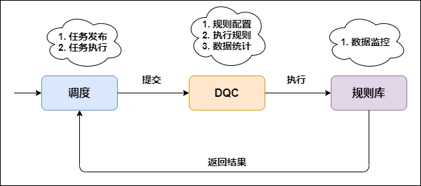
DQC data monitoring rules include strong rules and weak rules:
-
Strong rule: once the alarm is triggered, the execution of the task will be blocked (set the task to the failed state so that the downstream task will not be triggered for execution).
-
Weak rule: only alarm but not block the execution of tasks.
DQC provides common rule templates, including the volatility of table rows compared with N days ago, the volatility of table space compared with N days ago, the volatility of field maximum / minimum / average compared with N days ago, and the number of field null values / unique values.
In fact, DQC check is also a running SQL task, but this task is nested in the main task. Once there are too many checkpoints, it will naturally affect the overall performance. Therefore, it still depends on the data production level to determine the configuration of rules. For example, the monitoring rate of L1 and L2 data should reach more than 90%, and three or more rule types are required, while unimportant data assets are not mandatory.
2) Data timeliness monitoring
On the premise of ensuring the accuracy of data, it is necessary to further enable data to provide services in time, otherwise the value of data will be greatly reduced or even worthless. Therefore, ensuring data timeliness is also the top priority to ensure data quality.
- Task priority:
For the scheduling task of DataWorks platform, the priority can be set through the intelligent monitoring tool. The scheduling of DataWorks is a tree structure. When the priority of leaf node is configured, this priority will be passed to all upstream nodes, and leaf node is usually the consumption node of service business.
Therefore, in priority setting, we should first determine the asset level of the business. The higher the level of business, the higher the priority of the corresponding consumption node. We should give priority to scheduling and occupying computing resources to ensure the on-time output of high-level business.
In short, it is to give priority to the scheduling task of high-level data assets according to the level of data assets, and give priority to ensuring the data needs of high-level businesses.
- Task alarm:
The task alarm is similar to the priority. It is configured through the intelligent monitoring tool of DataWorks. Only the leaf node needs to be configured to transmit the alarm configuration to the upstream. Errors or delays may occur during task execution. In order to ensure the output of the most important data (i.e. data with high asset level), errors need to be handled immediately and delays need to be handled.
- DataWorks intelligent monitoring:
When DataWorks schedules offline tasks, it provides intelligent monitoring tools to monitor and alarm the scheduled tasks. According to the monitoring rules and task operation, intelligent monitoring makes decisions on whether to alarm, when to alarm, how to alarm and who to alarm. Intelligent monitoring will automatically select the most reasonable alarm time, alarm mode and alarm object.
4. Finally
To truly solve the problem of data quality, it is necessary to clarify the business needs, control the data quality from the needs, and establish a data quality management mechanism. Define the problem from the perspective of business. The tool automatically and timely finds the problem, defines the person responsible for the problem, and notifies the person responsible through e-mail, SMS and other means to ensure that the problem is notified to the person responsible in time. Track the progress of problem rectification and ensure the management of the whole process of data quality problems.
9, Guidelines for standardized construction of data warehouse
1. Code for public development of digital warehouse
1. Hierarchy calling specification
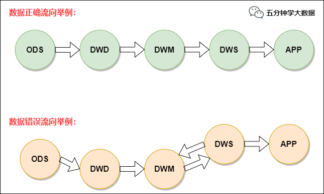
The stable business is developed according to the standard data flow, namely ODS – > DWD – > DWS – > app. Unstable business or exploratory requirements can follow the two model data flows of ODS - > DWD - > app or ODS - > DWD - > DWM - > app.
After ensuring the rationality of the data link, the layered reference principle of the model must also be guaranteed:
-
Normal flow direction: ODS - > DWD - > DWM - > DWS - > app. When the relationship of ODS - > DWD - > DWS - > app appears, it indicates that the subject field is not covered completely. DWD data should be dropped into DWM, and DWD - > DWS is allowed for tables with very low frequency of use.
-
Try to avoid tables in DWS wide tables that use DWD and DWM (the subject domain to which the DWD belongs).
-
In principle, DWM tables generated by DWM in the same subject domain should be avoided as much as possible, otherwise it will affect the efficiency of ETL.
-
Direct use of ODS tables is prohibited in DWM, DWS and APP. ODS tables can only be referenced by DWD.
-
Reverse dependencies are prohibited. For example, DWM tables depend on DWS tables.
give an example:
2. Data type specification
The data types of different data shall be uniformly specified, and the specified data types shall be strictly followed:
-
Amount: double or use decimal(11,2) to control accuracy, etc. to clarify whether the unit is minute or yuan.
-
String: string.
-
id class: bigint.
-
Time: string.
-
Status: string
3. Data redundancy specification
The redundant fields of the wide table should ensure that:
-
High frequency shall be used for redundant fields, and 3 or more downstream fields shall be used.
-
The introduction of redundant fields should not cause too much delay in their own data.
-
The repetition rate of redundant fields and existing fields should not be too large. In principle, it should not exceed 60%. If necessary, you can choose to join or expand the original table.
4. NULL field processing specification
-
For dimension fields, it needs to be set to - 1
-
For the indicator field, it needs to be set to 0
5. Specification of index caliber
Ensure that the indicators within the subject area are consistent and unambiguous.
Through data layering, provide unified data export and unified data caliber for external output, so as to avoid the occurrence of different caliber of the same index.
1) Index combing
The inconsistency of indicator caliber makes the cost of data use extremely high, and the problems of caliber fighting and cross checking data often occur. In data governance, we further sort out all the indicators we need to sort out and clarify their caliber. If there are two indicators with the same name but different caliber, first judge whether they are merged. If they need to exist at the same time, they must be able to be distinguished in naming.
2) Index management
Indicator management is divided into atomic indicator maintenance and derived indicator maintenance.
Atomic index:
- Select the production line, business segment, data field and business process to which the atomic indicator belongs
- The statistical data of the selected atomic indicator comes from the original data source under the business process
- Enter the English name, Chinese name and overview of atomic indicators
- Fill in index function
- The system automatically generates the definition expression of atomic index according to the index function
- The system generates atomic indicator SQL according to indicator definition expression and data source table
Derived indicators:
- On the basis of atomic indicators, some dimensions or modifier qualifiers are selected.
6. Data sheet processing specification
1) Incremental table
New data. Incremental data is the new data after the last export.
-
Record the amount of each increase, not the total amount;
-
The increment table only reports the change, and there is no need to report if there is no change;
-
One partition per day.
2) Full scale
All the latest status data every day.
-
The full scale shall be reported whether there is any change;
-
The data reported each time is all data (changed + unchanged);
-
There is only one partition.
3) Snapshot table
Divide by day and record the full amount of data as of the data date.
-
The snapshot table shall be reported whether there is any change;
-
The data reported each time is all data (changed + unchanged);
-
One partition a day.
4) Zipper Watch
Record the full amount of data as of the data date.
-
Record the information of all changes of a thing from the beginning to the current state;
-
Each time the zipper table reports the final status of the history record, which is the total amount of history recorded at the current time;
-
The current record stores the last change (total amount) of all historical records before the current time;
-
There is only one partition.
7. Table life cycle management
This part is mainly to generate the corresponding life cycle management matrix through the classification of historical data and table types.
1) Historical data classification
The historical data is mainly divided into four levels: P0, Pl, P2 and P3, which are specifically defined as follows:
-
P0: very important subject domain data and very important application data, which are irrecoverable, such as transaction, log, group KPI data and IPO association table.
-
Pl: important business data and important application data, which are irrecoverable, such as important business product data.
-
P2: important business data and important application data, with recoverability, such as intermediate process data generated by transaction line ETL.
-
P3: unimportant business data and unimportant application data are recoverable, such as some SNS product reports.
2) Table type division
- Event type flow table (incremental table)
Event type flow table (incremental table) refers to data without duplication or primary key, such as log.
- Event type image table (incremental table)
Event type image table (incremental table) refers to business process data. It has a primary key, but the attributes of the same primary key will change slowly. For example, the transaction, order status and time will change according to the business.
- Dimension table
Dimension tables include dimension and dimension attribute data, such as user tables and commodity tables.
- Merge full scale
The Merge full scale includes business process data or dimension table data. Because the data itself is newly added or the status changes, multiple copies of the data with the same primary key may be retained. Therefore, you can Merge these data according to the primary key. The attributes corresponding to the primary key will only retain the latest status, and the historical status will be retained in the partition of the previous day. For example, user tables and transaction tables can be merged.
- ETL temporary table
ETL temporary table refers to the temporary table data generated during ETL processing. It is generally not recommended to keep it for up to 7 days.
- TT temporary data
The data pulled by TT and the temporary data generated by DbSync will eventually flow to the DS layer, and the ODS layer data will be retained as the original data, making the upstream data of TT & DbSync become temporary data. This kind of data is not recommended to be retained for a long time. The life cycle is set to 93 days by default. The retention days can be appropriately reduced according to the actual situation.
7. General full scale
For many small business data or product data, BI generally pulls them directly in full. This method is efficient and does not have a great pressure on storage. Moreover, the table is retained for a long time. The retention policy can be determined according to the historical data level.
Through the above historical data level division and table type division, the corresponding life cycle management matrix is generated, as shown in the following table:
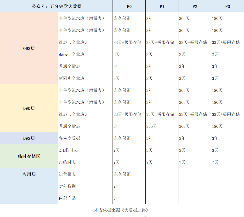
2. Development specification of each layer of data warehouse
1. Design specification for ODS layer
Synchronization specification:
-
A system source table can only be synchronized once;
-
The logic of full initialization synchronization and incremental synchronization shall be clear;
-
Partition storage based on statistical date and time;
-
The target table field should be automatically populated when the source table does not exist.
Table classification and life cycle:
- ods total flow meter:
-
Non renewable permanent preservation;
-
The log can be kept according to the requirements;
-
Set and retain special date data as required;
-
Set and retain special month data as required;
- ods mirror full scale:
-
It is recommended to store by day;
-
Preserve historical changes;
-
The latest data is stored in the largest partition;
-
Historical data shall be retained as required;
- ods incremental data:
-
It is recommended to store by day;
-
If there is a corresponding full scale, it is recommended to retain only 14 days of data;
-
If there is no corresponding full scale, it shall be retained permanently;
- Temporary table in etl process of ods:
-
It is recommended to keep it on demand;
-
Retain for up to 7 days;
-
It is recommended to delete it when it is used up and generate it next time;
- BDSync non deduplication data:
- It is reserved through the middle tier. It is deleted when used up by default. It is not recommended to keep it.
Data quality:
-
The full scale must be configured with unique field identification;
-
Monitor the partition empty data;
-
Monitor the change and distribution of enumeration values for enumeration type fields;
-
The data magnitude and record number of ods table are monitored month on month;
-
All ods tables must be annotated;
2. Design specification for public dimension layer
1) Design criteria
- uniformity
The field names, data types and data contents of common dimensions in different physical tables must be consistent (for historical reasons, version control should be done well)
- Combination and splitting of dimensions
- Combination principle:
Combine dimensions with highly related fields, query and display them together. The two dimensions must have a natural relationship, such as the basic attribute of goods and the brand to which they belong.
No relevance: for example, for some miscellaneous dimensions that are used less frequently, you can build a collection of special attributes of miscellaneous dimensions.
Behavior dimension: the calculated measurement, but the downstream dimension is processed. For example, the number of hits is 0-1000, 100-1000, etc., which can be aggregated and classified.
- Splitting and redundancy:
For importance, business relevance, source and usage frequency can be divided into core table and extended table.
For the larger dimension of data records, some subsets can be appropriately redundant.
2) Storage and lifecycle management
It is recommended to partition by day.
- When the maximum access span within 3 months is < = 4 days, it is recommended to retain the partition for the last 7 days;
- When the maximum access span within 3 months is < = 12 days, it is recommended to retain the partition for the last 15 days;
- When the maximum access span within 3 months is < = 30 days, it is recommended to retain the partition for the last 33 days;
- When the maximum access span within 3 months is < = 90 days, it is recommended to retain the partition for the last 120 days;
- When the maximum access span within 3 months is < = 180 days, it is recommended to retain the partition for the last 240 days;
- When the maximum access span within 3 months is < = 300 days, it is recommended to retain the partition for the last 400 days;
3. DWD detail layer design specification
1) Storage and lifecycle management
It is recommended to partition by day.
- When the maximum access span within 3 months is < = 4 days, it is recommended to retain the partition for the last 7 days;
- When the maximum access span within 3 months is < = 12 days, it is recommended to retain the partition for the last 15 days;
- When the maximum access span within 3 months is < = 30 days, it is recommended to retain the partition for the last 33 days;
- When the maximum access span within 3 months is < = 90 days, it is recommended to retain the partition for the last 120 days;
- When the maximum access span within 3 months is < = 180 days, it is recommended to retain the partition for the last 240 days;
- When the maximum access span within 3 months is < = 300 days, it is recommended to retain the partition for the last 400 days;
2) Design criteria of transactional fact table
-
Based on the analysis and design of data application requirements, the transactional fact table can be built based on an event process in combination with the larger downstream requirements for a business process and analysis indicators;
-
Generally, the date or time of the event is selected as the partition field to facilitate scanning and clipping;
-
The redundant subset principle is conducive to reducing the subsequent IO overhead;
-
The dimension of the detail level fact table is degraded to reduce the cost of subsequent use of the join.
3) Periodic snapshot fact table
-
Each row in the period snapshot fact table summarizes multiple measurement events that occur in a standard period, such as a day, a week, and a month.
-
Granularity is periodic, not individual transactions.
-
It usually contains many facts, because any measurement event consistent with the granularity of the fact table is allowed.
4) Cumulative snapshot fact table
-
A fact table constructed through the joint analysis of multiple business processes, such as the flow link of a purchase order.
-
Used to analyze the event time and the interval period between times.
-
A small number of statistics that are not supported by the current transaction type, such as closing, shipment and other related statistics.
4. Design specification for DWS public summary floor
The performance of data warehouse is one of the important criteria for the success of data warehouse construction. Aggregation is mainly used to improve query performance by summarizing detailed granularity data. By accessing the aggregated data, the workload that the database must perform in response to the query can be reduced, the query of users can be responded quickly, and the inconsistency of results caused by accessing detailed data by different users can be reduced.
1) Basic principles of aggregation
-
uniformity. The aggregation table must provide query results consistent with the query detail granularity data.
-
Avoid single table design. Do not store different levels of aggregated data in the same table.
-
Aggregation granularity can be different. Aggregation does not need to maintain the same granularity as the original fine-grained data. Aggregation only cares about the dimension of the query.
2) Basic steps of aggregation
Step 1: determine the aggregation dimension
In the original detail model, there will be multiple dimensions describing facts, such as date, commodity category, seller, etc. at this time, you need to determine what dimension to aggregate according to. If you only care about the transaction amount of commodities, you can aggregate data according to the commodity dimension.
Step 2: determine the consistency of drilling
At this time, you should be concerned about whether to summarize by month or by day, by commodity or by category. If you summarize by category, you also need to be concerned about whether to summarize by major category or minor category. Of course, all we have to do is understand what users need, and then aggregate according to what they want.
Step 3: determine the aggregation facts
In the original detailed model, there may be multiple fact measures, such as transaction volume and transaction quantity in the transaction. At this time, it is necessary to clarify whether to summarize according to transaction volume or transaction quantity.
3) Design principle of public summary floor
In addition to the basic principle of aggregation, the public aggregation layer must also follow the following principles:
-
Data commonality. Will the aggregation of summary be used by a third party? Is aggregation based on a certain dimension often used in data analysis? If the answer is yes, it is necessary to summarize and precipitate the detailed data into the aggregation table.
-
Do not cross data fields. Data domain is an abstraction that classifies and aggregates data at a higher level. If business
-
Distinguish statistical periods. The statistical period of data shall be explained in the naming of the table, such as_ Id indicates the last day_ td means as of the day_ nd indicates the last N days.
3. Naming standard of data warehouse
1. Root design specification
The root word belongs to the specification in the construction of data warehouse and belongs to the category of metadata management. Now it is classified as a part of data governance. The complete data warehouse construction includes data governance, but now when it comes to data warehouse, it is biased towards data modeling, while when it comes to data governance, it is more about data specification and data management.
Table naming is actually a reflection of metadata description to a great extent. The more perfect the table naming specification is, the more information we can get from the table name. For example, part of the business is about shelves. The English name is: rack. Rack is a root word. Then we call it rack in all tables, fields and other places. Don't call it anything else. This is the function of word root, which is used to name uniformly and express the same meaning.
There are many "rate" indicators in the index system, which can be disassembled into XXX+rate. The rate can be called rate, so all our indicators are called XXX+rate.
Root word: it can be used to unify table name, field name, subject domain name, etc.
For example: it is more intuitive and easy to understand to display in the form of flow chart. This figure focuses on the naming standard of dwm layer table, and other naming principles are similar:
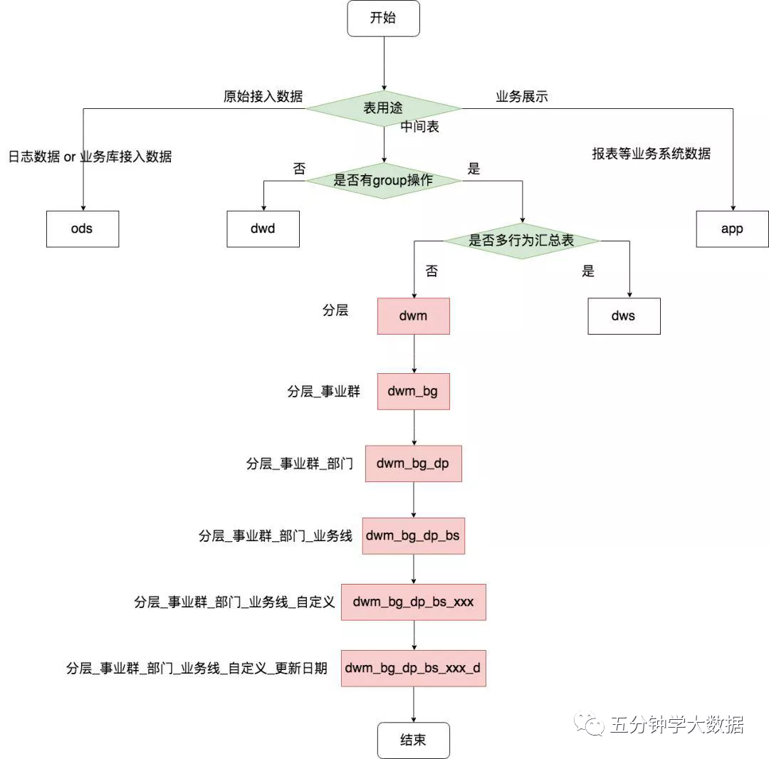
The first judgment condition is the purpose of the table, whether it is an intermediate table, an original log or a table for business display. If the table is judged as an intermediate table, it will go to the next judgment condition: whether the table has a group operation. Judge whether the table is divided into dwd layer or dwm and dws layer by whether there is a group operation. If it is not dwd layer, You need to judge whether the table is a summary table (i.e. wide table) of multiple behaviors, and then fill in the business group, Department, business line, user-defined name, update frequency and other information respectively.
Hierarchy: scope of use of tables
Business group and department: the team that produces the table or the data
Business line: indicates which product or business line the data is related to
Subject area: analyze the perspective of the problem, object and entity
User defined: generally, the information of this table will be described as much as possible, such as active table, retained table, etc
Update cycle: for example, day level or month level update
The naming specification of data warehouse table is as follows:
1. Warehouse level:
Common dimension: dim
DM layer: DM
ODS layer: ODS
DWD layer: DWD
DWS layer: DWS
2. Cycle / data range:
Daily snapshot: d
Increment: i
Total quantity: f
Zhou: w
Zipper Watch: l
Non divisional total scale: a
2. Table naming specification
1) General table
A regular table is a table that we need to solidify, a formal table, and a table that needs to be maintained and improved for a period of time.
Specification: hierarchical prefix [dwd|dws|ads]_ Department_ Business domain_ Subject domain_ XXX_ Update cycle | data range
We can enumerate the business domain and subject domain in the way of word root and constantly improve them.
The update cycle mainly includes time granularity, day, month, year, week, etc.
2) Intermediate table
Intermediate tables generally appear in a Job. They are tables of intermediate data temporarily stored in the Job. The scope of the intermediate table is limited to the current Job execution process. Once the Job is completed, the mission of the intermediate table is completed and can be deleted (you can choose freely according to your company's scenario. Previously, the company would keep the intermediate table data for several days for troubleshooting).
Specification: mid_table_name_[0~9|dim]
table_name is the name of the target table in our task. Generally speaking, a task has only one target table. The purpose of adding the table name here is to prevent the conflict of table names during free play. At the end, you can choose to play freely and give some meaningful names, or simply and rudely use numbers instead. Each has its own advantages and disadvantages. Choose carefully.
Usually, you will encounter a table that needs to complete the dimension. Here, you end with dim.
If you want to keep the middle table of history, you can add a date or time stamp.
3) Temporary table
Temporary tables are temporary test tables, which are used once temporarily. They are tables that can be deleted at any time. They are tables that are no longer used in the future.
Specification: tmp_xxx
As long as you start with tmp, other names are optional. Note that the table starting with tmp should not be used for actual use, but only for test and verification.
4) Dimension table
Dimension table is an abstract table describing classes based on underlying data. Dimension tables can be abstracted from the underlying tables automatically or maintained manually.
Specification: dim_xxx
The dimension table starts with dim, followed by the description of the indicator.
5) Manual table
Manual tables are manually maintained tables. After manual initialization, they will not be changed automatically. Subsequent changes are also maintained manually.
Generally speaking, the granularity of manual data is too fine, so it is temporarily placed in the dwd layer. If there are target values or other types of manual data, it will be layered according to the actual situation.
Specification: dwd_ Business domain_ manual_xxx
Manual table: add a special topic field, manual, to indicate manual maintenance of the table.
3. Index naming standard
Public rules
-
All words in lowercase
-
Underline segmentation between words (counterexample: AppName or AppName)
-
Readability is better than length (root word, avoiding the same index, naming consistency)
-
It is forbidden to use sql keywords, such as + col when the field name conflicts with the keyword
-
Quantity field suffix_ cnt and other identification
-
Amount field suffix_ price identification
-
The day partition uses the field dt in a unified format (yyyymmdd or yyyy MM DD)
-
Hour partition use field hh, range (00-23)
-
Minute partition use field mi, range (00-59)
-
Boolean type identifier: is_ {business}, null value is not allowed
Reference documents:
- Hundreds of high-quality big data books with a required reading list (big data treasure)
- The strongest and most comprehensive standard guide for data warehouse construction
- Meituan data platform and data warehouse construction practice, over 100000 words summary
- 50000 words | it took a month to sort out this Hadoop blood spitting dictionary