abstract

Based on the prediction of the accommodation reservation results of new Airbnb users, this paper completely describes the whole process from data exploration to feature engineering to model construction. Project address: Airbnb New User Bookings | Kaggle
Of which:
1. The data exploration part is mainly based on pandas library, using the common: head(), value_ Count(), describe(), isnull(), unique() and other functions, as well as understanding and exploring the data through matplotlib mapping;
2. The feature engineering part mainly extracts the year, month, day, season and weekday from the date, segments the age, calculates the difference between relevant features, and groups them according to the user id, so as to count the times, average value, standard deviation, etc. of some feature variables, and encode the data through one hot encoding and labels encoding to extract features;
3. The model construction part is mainly based on the sklearn package and xgboost package, which is predicted by calling different models. The models involved include: Logistic Regression model, Logistic Regression model, tree model: DecisionTree, RandomForest, AdaBoost, Bagging, ExtraTree, GraBoost, SVM model: SVM RBF, SVM poly, SVM linear, xgboost, And by changing the parameters and data size of the model to observe the scoring results of NDCG, so as to understand the impact of different models, parameters and data size on the prediction results

1. Background

About this Dataset,In this challenge, you are given a list of users along with their demographics, web session records, and some summary statistics. You are asked to predict which country a new user's first booking destination will be. All the users in this dataset are from the USA.

There are 12 possible outcomes of the destination country: 'US', 'FR', 'CA', 'GB', 'ES', 'IT', 'PT', 'NL','DE', 'AU', 'NDF' (no destination found), and 'other'. Please note that 'NDF' is different from 'other' because 'other' means there was a booking, but is to a country not included in the list, while 'NDF' means there wasn't a booking.

2. Data description

A total of 6 csv files are included

1. train_users_2.csv - the training set of users
2. test_users.csv - the test set of users

1. id: user id
2. date_account_created (account registration time): the date of account creation
3. timestamp_first_active: timestamp of the first activity, note that it can be earlier than date_account_created or date_first_booking because a user can search before signing up
4. date_first_booking time: date of first booking
5. gender
6. age
7. signup_method (registration method)
8. signup_flow: the page a user come to sign up from
9. Language: international language preference
10. affiliate_channel: what kind of paid marketing
11. affiliate_provider: where the marketing is e.g. google, craigslist, other
12. first_affiliate_tracked: what the first marketing the user interacted with before the signing up
13. signup_app (register app)
14. first_ device_ Type (device type)
15. first_browser (browser type)
16. country_destination: this is the target variable you are to predict

3. sessions.csv - web sessions log for users

1. user_id (user id): to be joined with the column 'id' in users table
2. Action (user behavior)
3. action_type (user behavior type)
4. action_detail (specific user behavior)
5. device_type (device type)
6. secs_elapsed (length of stay)

4. sample_submission.csv - correct format for submitting your predictions

import numpy as np
import pandas as pd
import matplotlib.pyplot as plt
import sklearn as sk
%matplotlib inline
import datetime
import os
import seaborn as sns#Data visualization
from datetime import date
from sklearn.preprocessing import LabelEncoder
from sklearn.preprocessing import StandardScaler
from sklearn.preprocessing import LabelBinarizer
import pickle #For storing models
import seaborn as sns
from sklearn.metrics import *
from sklearn.model_selection import *

3. Data exploration

• Based on Jupiter notebook and python 3

3.1 train_users_2 and test_users file

3.1.1 reading files

train = pd.read_csv("train_users_2.csv")
test = pd.read_csv("test_users.csv")

3.1.2 import package

import numpy as np
import pandas as pd
import matplotlib.pyplot as plt
import sklearn as sk
%matplotlib inline
import datetime
import os
import seaborn as sns#Data visualization
from datetime import date
from sklearn.preprocessing import LabelEncoder
from sklearn.preprocessing import StandardScaler
from sklearn.preprocessing import LabelBinarizer
import pickle #For storing models
import seaborn as sns
from sklearn.metrics import *
from sklearn.model_selection import *

3.1.3 viewing data includes the following features:

print('the columns name of training dataset:\n',train.columns)
print('the columns name of test dataset:\n',test.columns)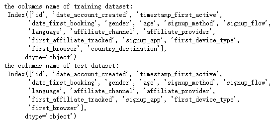

Analysis:

1. The train file has more features than the test file - country_destination
2. country_destination is the target variable to be predicted
3. During data exploration, focus on analyzing the train file, which is similar to the test file

3.1.4 viewing data information:

print(train.info())

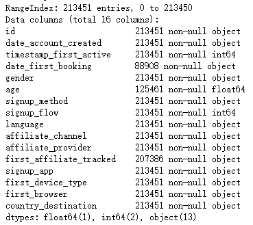
analysis:

1. trian file contains 213451 lines of data and 16 features
2. Data type and non null value of each feature
3. date_first_booking has many null values, which can be considered to be deleted during feature extraction

3.1.5 characteristic analysis:

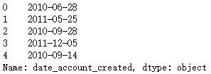
date_account_created

① View date_account_created previous rows of data

print(train.date_account_created.head())

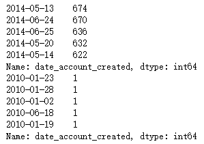
② Yes, date_ account_ Create data for statistics

print(train.date_account_created.value_counts().head())
print(train.date_account_created.value_counts().tail())

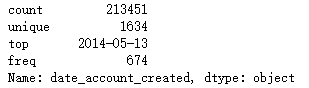
③ Get date_account_created information

print(train.date_account_created.describe())

④ Observe user growth

dac_train = train.date_account_created.value_counts()
dac_test = test.date_account_created.value_counts()
#Convert data type to datatime type
dac_train_date = pd.to_datetime(train.date_account_created.value_counts().index)
dac_test_date = pd.to_datetime(test.date_account_created.value_counts().index)
#Calculate the number of days from the time of first registration
dac_train_day = dac_train_date - dac_train_date.min()
dac_test_day = dac_test_date - dac_train_date.min()
#motplotlib mapping
plt.scatter(dac_train_day.days, dac_train.values, color = 'r', label = 'train dataset')
plt.scatter(dac_test_day.days, dac_test.values, color = 'b', label = 'test dataset')

plt.title("Accounts created vs day")
plt.xlabel("Days")
plt.ylabel("Accounts created")
plt.legend(loc = 'upper left')

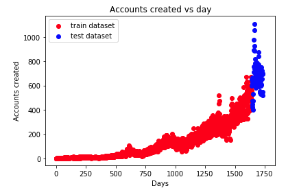
analysis:

1. x-axis: the number of days from the time of first registration
2. y-axis: number of users registered on the same day
3. With the growth of time, the number of user registrations is rising sharply

timestamp_first_active
① View the first few rows of data

print(train.timestamp_first_active.head())

Analysis: the result [1] shows that timestamp_first_active has no duplicate data

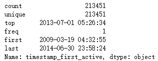
② Convert the time stamp into date form and obtain data information

tfa_train_dt = train.timestamp_first_active.astype(str).apply(lambda x:  
                                                                    datetime.datetime(int(x[:4]),
                                                                                      int(x[4:6]), 
                                                                                      int(x[6:8]), 
                                                                                      int(x[8:10]), 
                                                                                      int(x[10:12]),
                                                                                      int(x[12:])))
print(tfa_train_dt.describe())

date_first_booking
① Get data information

print(train.date_first_booking.describe())
print(test.date_first_booking.describe())

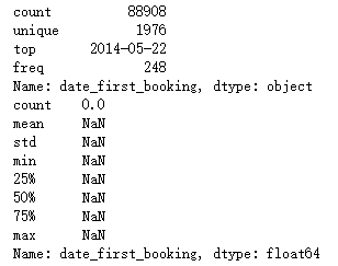
analysis:

1. Date in train file_ first_ Booking has a large number of missing values
2. Date in test file_ first_ Bookings are all missing values
3. Feature date can be deleted_ first_ booking

4.age
① Statistics of data

print(train.age.value_counts().head())

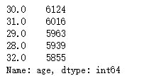
Analysis: the age of users is mainly about 30
② Histogram statistics

#Firstly, age was divided into four groups: missing values, too small age, reasonable age and too large age
age_train =[train[train.age.isnull()].age.shape[0],
            train.query('age < 15').age.shape[0],
            train.query("age >= 15 & age <= 90").age.shape[0],
            train.query('age > 90').age.shape[0]]

age_test = [test[test.age.isnull()].age.shape[0],
            test.query('age < 15').age.shape[0],
            test.query("age >= 15 & age <= 90").age.shape[0],
            test.query('age > 90').age.shape[0]]

columns = ['Null', 'age < 15', 'age', 'age > 90']

# plot
fig, (ax1,ax2) = plt.subplots(1,2,sharex=True, sharey = True,figsize=(10,5))

sns.barplot(columns, age_train, ax = ax1)
sns.barplot(columns, age_test, ax = ax2)

ax1.set_title('training dataset')
ax2.set_title('test dataset')
ax1.set_ylabel('counts')

 

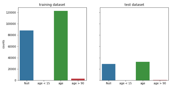
Analysis: the abnormal age is less, and there are a certain number of missing values

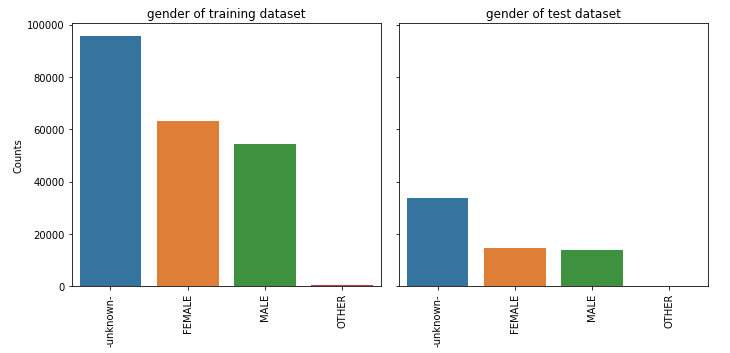
Other features

• Because there are few labels for other features in the train file, we can directly carry out one hot encoding in the feature engineering

The histogram is used uniformly for statistics

def feature_barplot(feature, df_train = train, df_test = test, figsize=(10,5), rot = 90, saveimg = False): 
    feat_train = df_train[feature].value_counts()
    feat_test = df_test[feature].value_counts()
    fig_feature, (axis1,axis2) = plt.subplots(1,2,sharex=True, sharey = True, figsize = figsize)
    sns.barplot(feat_train.index.values, feat_train.values, ax = axis1)
    sns.barplot(feat_test.index.values, feat_test.values, ax = axis2)
    axis1.set_xticklabels(axis1.xaxis.get_majorticklabels(), rotation = rot)
    axis2.set_xticklabels(axis1.xaxis.get_majorticklabels(), rotation = rot)
    axis1.set_title(feature + ' of training dataset')
    axis2.set_title(feature + ' of test dataset')
    axis1.set_ylabel('Counts')
    plt.tight_layout()
    if saveimg == True:
        figname = feature + ".png"
        fig_feature.savefig(figname, dpi = 75)

① gender

feature_barplot('gender', saveimg = True)

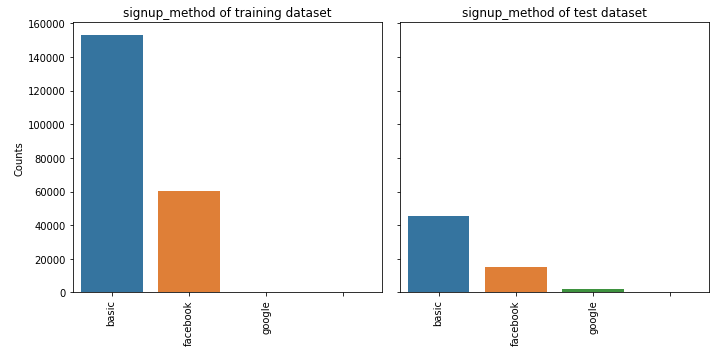
② signup_method

feature_barplot('signup_method')

③ signup_flow

feature_barplot('signup_flow')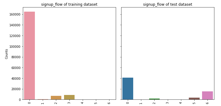

 

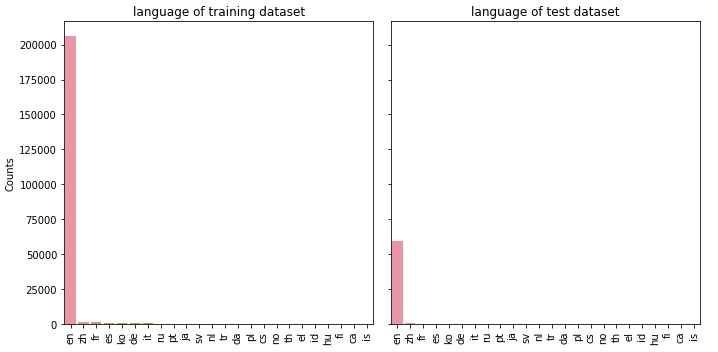
④ language

feature_barplot('language')

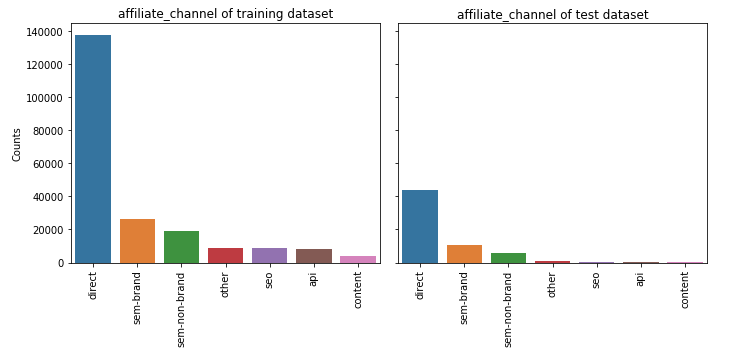
⑤ affiliate_channel

feature_barplot('affiliate_channel')

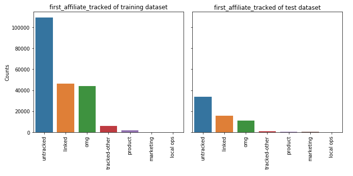
⑥ first_affiliate_tracked

feature_barplot('first_affiliate_tracked')

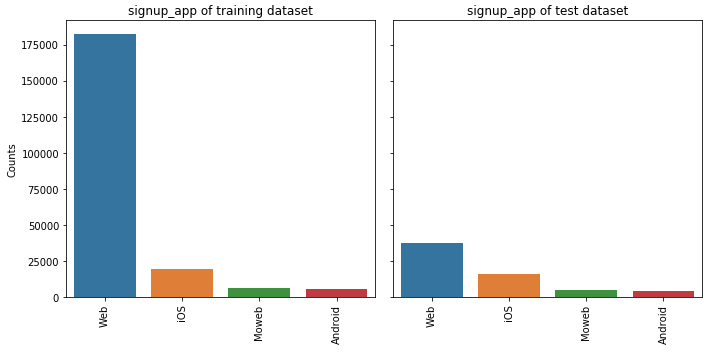
⑦ signup_app

feature_barplot('signup_app')

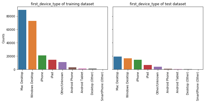
⑧ first_device_type

feature_barplot('first_device_type')

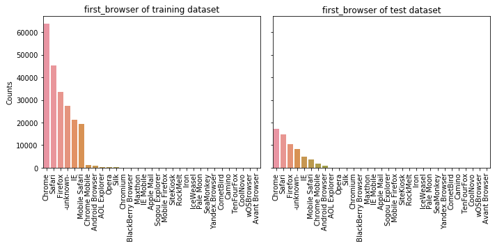
⑨ first_browser

feature_barplot('first_browser')

 

3.2 session data

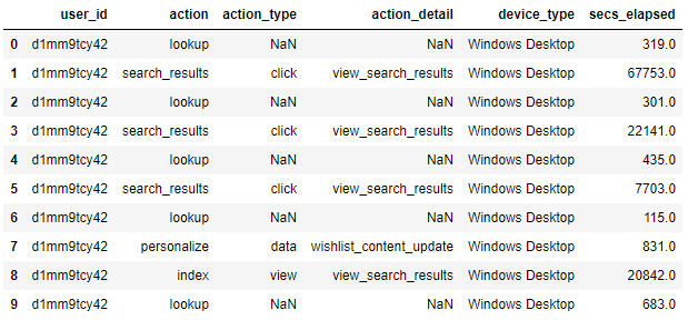
#Get the data and look up the first 10 rows of data
df_sessions = pd.read_csv('sessions.csv')
df_sessions.head(10)

3.2.1 user_id renamed id

#This is for later data consolidation
df_sessions['id'] = df_sessions['user_id']
df_sessions = df_sessions.drop(['user_id'],axis=1) #Delete by line

3.2.2 view data shape

df_sessions.shape

(10567737, 6)
Analysis: the session file has 10567737 lines of data and 6 features

3.2.3 viewing missing values

df_sessions.isnull().sum()

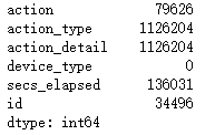
Analysis: action, action_type，action_detail， secs_elapsed has many missing values

3.2.4 fill in missing values

df_sessions.action = df_sessions.action.fillna('NAN')
df_sessions.action_type = df_sessions.action_type.fillna('NAN')
df_sessions.action_detail = df_sessions.action_detail.fillna('NAN')
df_sessions.isnull().sum()

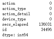
analysis:

1. The missing value after filling has been 0
2. secs_elapsed is filled in later

4. Feature extraction

• After having a certain understanding of the data, we carry out feature extraction

4.1 feature extraction of session file

4.1.1 action

df_sessions.action.head()

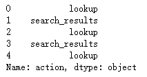
df_sessions.action.value_counts().min()

1
Analysis: according to the statistics of actions, we can find that there are many kinds of user actions, and the minimum number of occurrences is only 1. Next, we can list the behaviors with less occurrences as OTHER

① List the characteristic action s whose times are lower than the threshold value of 100 as OTHER

#Action values with low frequency are changed to 'OTHER'
act_freq = 100  #Threshold of frequency
act = dict(zip(*np.unique(df_sessions.action, return_counts=True)))
df_sessions.action = df_sessions.action.apply(lambda x: 'OTHER' if act[x] < act_freq else x)
#np.unique(df_sessions.action, return_counts=True) returns the non repeated action value and its quantity in the form of array
#Zip (* (a,b)) a and B elements correspond one to one and return zip object

② Action on feature_ detail，action_type，device_type，secs_elapsed for refinement

• Firstly, the characteristics of users are grouped according to user id
• **Characteristic action: * * count the total number of actions per user, the number of each action type, average value and standard deviation
• **Feature action_detail: * * count the total actions of each user_ Number of occurrences of detail, each action_ Number, mean and standard deviation of detail type
• **Feature action_type: * * count the total actions of each user_ Number of occurrences of type, each action_ Number, average, standard deviation and total residence time of type (log processing)
• **Feature device_type: * * count the total devices of each user_ Number of occurrences of type, each device_ Number of type types, mean and standard deviation
• **Characteristic secs_elapsed: * * fill the missing value with 0 and count secs of each user_ Sum, mean, standard deviation and median of elapsed time (log processing), (sum / mean), secs_elapsed (after log processing) number of occurrences at each time
   

#Refine the action feature
f_act = df_sessions.action.value_counts().argsort()
f_act_detail = df_sessions.action_detail.value_counts().argsort()
f_act_type = df_sessions.action_type.value_counts().argsort()
f_dev_type = df_sessions.device_type.value_counts().argsort()

#Group by id
dgr_sess = df_sessions.groupby(['id'])
#Loop on dgr_sess to create all the features.
samples = [] #samples list
ln = len(dgr_sess) #Calculate DF after grouping_ Length of sessions

for g in dgr_sess:  #To DGR_ The data of each id in sess is traversed
    gr = g[1]   #data frame that comtains all the data for a groupby value 'zzywmcn0jv'
    
    l = []  #Create an empty list to temporarily store features
    
    #the id    for example:'zzywmcn0jv'
    l.append(g[0]) #Put the id value into an empty list
    
    # number of total actions
    l.append(len(gr))#Put the length of the data corresponding to the id into the list
    
    #secs_ The missing value in the elapsed feature is filled with 0, and then the specific residence time value is obtained
    sev = gr.secs_elapsed.fillna(0).values   #These values are used later.
    
    #action features - user behavior 
    #The number of occurrences of each user's behavior, the number of each behavior type, the average value and the standard deviation
    c_act = [0] * len(f_act)
    for i,v in enumerate(gr.action.values): #i is the corresponding position from 0-1, and v is the value of user behavior characteristics
        c_act[f_act[v]] += 1
    _, c_act_uqc = np.unique(gr.action.values, return_counts=True)
    #Calculate the length, average value and standard deviation of each type of user behavior characteristics
    c_act += [len(c_act_uqc), np.mean(c_act_uqc), np.std(c_act_uqc)]
    l = l + c_act
    
    #action_detail features - specific user behavior
    #(how many times each value occurs, numb of unique values, mean and std)
    c_act_detail = [0] * len(f_act_detail)
    for i,v in enumerate(gr.action_detail.values):
        c_act_detail[f_act_detail[v]] += 1
    _, c_act_det_uqc = np.unique(gr.action_detail.values, return_counts=True)
    c_act_detail += [len(c_act_det_uqc), np.mean(c_act_det_uqc), np.std(c_act_det_uqc)]
    l = l + c_act_detail
    
    #action_type features - user behavior type click, etc
    #(how many times each value occurs, numb of unique values, mean and std
    #+ log of the sum of secs_elapsed for each value)
    l_act_type = [0] * len(f_act_type)
    c_act_type = [0] * len(f_act_type)
    for i,v in enumerate(gr.action_type.values):
        l_act_type[f_act_type[v]] += sev[i] #sev = gr.secs_elapsed.fillna(0).values, find the total residence time of each behavior type
        c_act_type[f_act_type[v]] += 1  
    l_act_type = np.log(1 + np.array(l_act_type)).tolist() #The total residence time of each behavior type is quite different, and log processing is carried out
    _, c_act_type_uqc = np.unique(gr.action_type.values, return_counts=True)
    c_act_type += [len(c_act_type_uqc), np.mean(c_act_type_uqc), np.std(c_act_type_uqc)]
    l = l + c_act_type + l_act_type    
    
    #device_type features - device type
    #(how many times each value occurs, numb of unique values, mean and std)
    c_dev_type  = [0] * len(f_dev_type)
    for i,v in enumerate(gr.device_type .values):
        c_dev_type[f_dev_type[v]] += 1 
    c_dev_type.append(len(np.unique(gr.device_type.values))) 
    _, c_dev_type_uqc = np.unique(gr.device_type.values, return_counts=True)
    c_dev_type += [len(c_dev_type_uqc), np.mean(c_dev_type_uqc), np.std(c_dev_type_uqc)]        
    l = l + c_dev_type    
    
    #secs_elapsed features - length of stay     
    l_secs = [0] * 5 
    l_log = [0] * 15
    if len(sev) > 0:
        #Simple statistics about the secs_elapsed values.
        l_secs[0] = np.log(1 + np.sum(sev))
        l_secs[1] = np.log(1 + np.mean(sev)) 
        l_secs[2] = np.log(1 + np.std(sev))
        l_secs[3] = np.log(1 + np.median(sev))
        l_secs[4] = l_secs[0] / float(l[1]) #
        
        #Values are grouped in 15 intervals. Compute the number of values
        #in each interval.
        #sev = gr.secs_elapsed.fillna(0).values 
        log_sev = np.log(1 + sev).astype(int)
        #np.bincount():Count number of occurrences of each value in array of non-negative ints.  
        l_log = np.bincount(log_sev, minlength=15).tolist()                    
    l = l + l_secs + l_log
    
    #The list l has the feature values of one sample.
    samples.append(l)

#preparing objects    
samples = np.array(samples) 
samp_ar = samples[:, 1:].astype(np.float16) #Get the characteristic data except id
samp_id = samples[:, 0]   #Take id, which is in the first column

#Create a dataframe for the extracted features     
col_names = []    #name of the columns
for i in range(len(samples[0])-1):  #The reason for subtracting 1 is because there is an id
    col_names.append('c_' + str(i))  #How to name    
df_agg_sess = pd.DataFrame(samp_ar, columns=col_names)
df_agg_sess['id'] = samp_id
df_agg_sess.index = df_agg_sess.id #Use id as index

df_agg_sess.head()

 

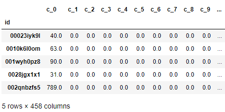
Analysis: after feature extraction, the session file changes from 6 features to 458 features

4.2 feature extraction of trian and test files

4.2.1 mark the number of lines in the train file and store the target variables we predict

• labels stores the target variable country for our prediction_ destination

train = pd.read_csv("train_users_2.csv")
test = pd.read_csv("test_users.csv")
#Calculate the number of lines of the train to facilitate the separation of the train and test data
train_row = train.shape[0]  

# The label we need to predict
labels = train['country_destination'].values

Delete date_ first_ Country in booking and train files_ destination

When we explore the data, we find date_first_booking is missing too many values in the train and test files, so it is deleted
Delete country_destination, use the model to predict the country_destination, and then with the stored country_ Compare the labels of destination to judge the advantages and disadvantages of the model

train.drop(['country_destination', 'date_first_booking'], axis = 1, inplace = True)
test.drop(['date_first_booking'], axis = 1, inplace = True)

4.2.2 merge train and test files

• It is convenient for the same feature extraction operation

#Connect test and train
df = pd.concat([train, test], axis = 0, ignore_index = True)

4.2.3  timestamp_first_active

① Convert to datetime type

tfa = df.timestamp_first_active.astype(str).apply(lambda x: datetime.datetime(int(x[:4]),
                                                                          int(x[4:6]), 
                                                                          int(x[6:8]),
                                                                          int(x[8:10]),
                                                                          int(x[10:12]),
                                                                          int(x[12:])))

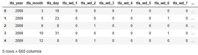
② Extracted features: year, month, day

# create tfa_year, tfa_month, tfa_day feature
df['tfa_year'] = np.array([x.year for x in tfa])
df['tfa_month'] = np.array([x.month for x in tfa])
df['tfa_day'] = np.array([x.day for x in tfa])

③ Extracting features: weekday

• Evaluate the results one hot encoding code

#isoweekday() can return the day of the week, e.g. Sunday: 0; Monday: 1
df['tfa_wd'] = np.array([x.isoweekday() for x in tfa]) 
df_tfa_wd = pd.get_dummies(df.tfa_wd, prefix = 'tfa_wd')  # one hot encoding 
df = pd.concat((df, df_tfa_wd), axis = 1) #Features after adding df['tfa_wd '] encoding
df.drop(['tfa_wd'], axis = 1, inplace = True)#Delete original uncoded features

④ Extracted features: Season

• Since the judgment of seasons focuses on the month, the year is unified

Y = 2000
seasons = [(0, (date(Y,  1,  1),  date(Y,  3, 20))),  #'winter'
           (1, (date(Y,  3, 21),  date(Y,  6, 20))),  #'spring'
           (2, (date(Y,  6, 21),  date(Y,  9, 22))),  #'summer'
           (3, (date(Y,  9, 23),  date(Y, 12, 20))),  #'autumn'
           (0, (date(Y, 12, 21),  date(Y, 12, 31)))]  #'winter'

def get_season(dt):
    dt = dt.date() #get date
    dt = dt.replace(year=Y) #Replace the year of unification with the year of 2000
    return next(season for season, (start, end) in seasons if start <= dt <= end)

df['tfa_season'] = np.array([get_season(x) for x in tfa])
df_tfa_season = pd.get_dummies(df.tfa_season, prefix = 'tfa_season') # one hot encoding 
df = pd.concat((df, df_tfa_season), axis = 1)
df.drop(['tfa_season'], axis = 1, inplace = True)

4.2.4 date_account_created

① Set date_account_created converted to datetime type

dac = pd.to_datetime(df.date_account_created)

② Extracted features: year, month, day

# create year, month, day feature for dac

df['dac_year'] = np.array([x.year for x in dac])
df['dac_month'] = np.array([x.month for x in dac])
df['dac_day'] = np.array([x.day for x in dac])

③ Extracting features: weekday

# create features of weekday for dac

df['dac_wd'] = np.array([x.isoweekday() for x in dac])
df_dac_wd = pd.get_dummies(df.dac_wd, prefix = 'dac_wd')
df = pd.concat((df, df_dac_wd), axis = 1)
df.drop(['dac_wd'], axis = 1, inplace = True)

④ Extracted features: Season

# create season features fro dac

df['dac_season'] = np.array([get_season(x) for x in dac])
df_dac_season = pd.get_dummies(df.dac_season, prefix = 'dac_season')
df = pd.concat((df, df_dac_season), axis = 1)
df.drop(['dac_season'], axis = 1, inplace = True)

⑤ Extracted feature: date_account_created and timestamp_ first_ Difference between active

• That is, the time spent by users from being active on the airbnb platform to officially registering

dt_span = dac.subtract(tfa).dt.days 

• dt_ The first ten rows of data in span

dt_span.value_counts().head(10)

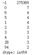
Analysis: the data is mainly concentrated in - 1. It can be guessed that users register DT on the same day_ The span value is - 1

• Extract features from the difference: the difference is one day, one month, one year and others
• That is, the time spent from user activity to registration is one day, one month, one year or other

# create categorical feature: span = -1; -1 < span < 30; 31 < span < 365; span > 365
def get_span(dt):
    # dt is an integer
    if dt == -1:
        return 'OneDay'
    elif (dt < 30) & (dt > -1):
        return 'OneMonth'
    elif (dt >= 30) & (dt <= 365):
        return 'OneYear'
    else:
        return 'other'

df['dt_span'] = np.array([get_span(x) for x in dt_span])
df_dt_span = pd.get_dummies(df.dt_span, prefix = 'dt_span')
df = pd.concat((df, df_dt_span), axis = 1)
df.drop(['dt_span'], axis = 1, inplace = True)

⑥ Delete existing features

• Yes, timestamp_first_active，date_ account_ After feature extraction, the original feature is deleted from the feature list

df.drop(['date_account_created','timestamp_first_active'], axis = 1, inplace = True)

4.2.5  age

#Age acquisition age
av = df.age.values

• In the data exploration stage, we found that most of the data were concentrated in the (15, 90) range, but some of the ages were distributed in the (19002000) range. We guessed that the user mistakenly filled in the date of birth as the age, so we preprocessed it

#This are birthdays instead of age (estimating age by doing 2014 - value)
#The data is from 2014, so 2014 value is used
av = np.where(np.logical_and(av<2000, av>1900), 2014-av, av) 
df['age'] = av

① Age segmentation

# Age has many abnormal values that we need to deal with. 
age = df.age
age.fillna(-1, inplace = True) #The null value is filled with - 1
div = 15
def get_age(age):
    # age is a float number
    if age < 0:
        return 'NA' #Indicates a null value
    elif (age < div):
        return div #If the age is less than 15 years old, return to 15 years old
    elif (age <= div * 2):
        return div*2 #If the age is greater than 15 and less than or equal to 30, 30 is returned
    elif (age <= div * 3):
        return div * 3
    elif (age <= div * 4):
        return div * 4
    elif (age <= div * 5):
        return div * 5
    elif (age <= 110):
        return div * 6
    else:
        return 'Unphysical' #Abnormal age

• Put the segmented age into the feature list as a new feature

df['age'] = np.array([get_age(x) for x in age])
df_age = pd.get_dummies(df.age, prefix = 'age')
df = pd.concat((df, df_age), axis = 1)
df.drop(['age'], axis = 1, inplace = True)

4.2.6 other features

• During data exploration, we found that the remaining feature labels are relatively few, so we do not further feature extraction, but only one hot encoding

feat_toOHE = ['gender', 
             'signup_method', 
             'signup_flow', 
             'language', 
             'affiliate_channel', 
             'affiliate_provider', 
             'first_affiliate_tracked', 
             'signup_app', 
             'first_device_type', 
             'first_browser']
#One hot encoding for other features
for f in feat_toOHE:
    df_ohe = pd.get_dummies(df[f], prefix=f, dummy_na=True)
    df.drop([f], axis = 1, inplace = True)
    df = pd.concat((df, df_ohe), axis = 1)

4.3 integrate all extracted features

• We will merge the features extracted from session, train and test files

#Integrate the features extracted from the session
df_all = pd.merge(df, df_agg_sess, how='left')
df_all = df_all.drop(['id'], axis=1) #id delete
df_all = df_all.fillna(-2)  #Processing missing values for features without session data

#A column is added to indicate the total number of null values in each row, which is also a feature
df_all['all_null'] = np.array([sum(r<0) for r in df_all.values]) 

5. Model construction

5.1 data preparation

5.1.1 separate train and test data

• train_row is the number of previously recorded train data rows

Xtrain = df_all.iloc[:train_row, :]
Xtest = df_all.iloc[train_row:, :]

5.1.2} generate the extracted features into csv files

Xtrain.to_csv("Airbnb_xtrain_v2.csv")
Xtest.to_csv("Airbnb_xtest_v2.csv")
#labels.tofile(): Write array to a file as text or binary (default)
labels.tofile("Airbnb_ytrain_v2.csv", sep='\n', format='%s') #Store target variables

• Read feature file

xtrain = pd.read_csv("Airbnb_xtrain_v2.csv",index_col=0)
ytrain = pd.read_csv("Airbnb_ytrain_v2.csv", header=None)
xtrain.head()

ytrain.head()

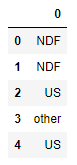
Analysis: it can be found that after feature extraction, the feature file xtrain is expanded to 665 features, and ytrain contains the target variables in the training set

5.1.3 label encoding target variables

le = LabelEncoder()
ytrain_le = le.fit_transform(ytrain.values)

• Before labels encoding: ['AU', 'CA', 'DE', 'ES',' FR ',' GB ',' IT ',' NDF ',' NL ',' PT ',' US', 'other']
• After labels encoding: [0, 1, 2, 3, 4, 5, 6, 7, 8, 9, 10, 11]

5.1.4} extract 10% of the data for model training

Reduce the time spent training the model

# Let us take 10% of the data for faster training. 
n = int(xtrain.shape[0]*0.1)
xtrain_new = xtrain.iloc[:n, :]  #Training data
ytrain_new = ytrain_le[:n]       #Target variables of training data

5.1.5 standard scaling dataset

Standardization of data sets is a common requirement of many machine learning estimators: if individual features do not look more or less like standard normal distribution data (for example, Gaussian with mean and unit variance of 0), they may perform poorly

X_scaler = StandardScaler()
xtrain_new = X_scaler.fit_transform(xtrain_new)

5.2 scoring model: NDCG

NDCG is an evaluation index to measure the ranking quality, which considers the correlation of all elements
Since the target variable we predict is not a binary variable, we use NDGG model to score the model and judge the advantages and disadvantages of the model
General dichotomous variables: we are used to using F1 score, precision, recall and AUC score to score the model

from sklearn.metrics import make_scorer

def dcg_score(y_true, y_score, k=5):
    
    """
    y_true : array, shape = [n_samples] #data
        Ground truth (true relevance labels).
    y_score : array, shape = [n_samples, n_classes] #Predicted score
        Predicted scores.
    k : int
    """
    order = np.argsort(y_score)[::-1] #Rank scores from high to low
    y_true = np.take(y_true, order[:k]) #Take out the first k[0,k) scores
      
    gain = 2 ** y_true - 1   

    discounts = np.log2(np.arange(len(y_true)) + 2)
    return np.sum(gain / discounts)
  

def ndcg_score(ground_truth, predictions, k=5):   

    """
    Parameters
    ----------
    ground_truth : array, shape = [n_samples]
        Ground truth (true labels represended as integers).
    predictions : array, shape = [n_samples, n_classes] 
        Predicted probabilities. Predicted probability
    k : int
        Rank.
    """
    lb = LabelBinarizer()
    lb.fit(range(len(predictions) + 1))
    T = lb.transform(ground_truth)    
    scores = []
    # Iterate over each y_true and compute the DCG score
    for y_true, y_score in zip(T, predictions):
        actual = dcg_score(y_true, y_score, k)
        best = dcg_score(y_true, y_true, k)
        score = float(actual) / float(best)
        scores.append(score)

    return np.mean(scores)

6. Build model

6.1 Logistic Regression

from sklearn.linear_model import LogisticRegression
from sklearn.model_selection import KFold
from sklearn.model_selection import cross_val_score
from sklearn.model_selection import train_test_split
lr = LogisticRegression(C = 1.0, penalty='l2', multi_class='ovr')
RANDOM_STATE = 2017  #Random seed

#k-fold cross validation
kf = KFold(n_splits=5, random_state=RANDOM_STATE) #Divided into 5 groups
train_score = [] 
cv_score = []

# select a k  (value how many y):
k_ndcg = 3 
# kf.split: Generate indices to split data into training and test set.
for train_index, test_index in kf.split(xtrain_new, ytrain_new):
    #The training set data is divided into training set and test set, and y is the target variable
    X_train, X_test = xtrain_new[train_index, :], xtrain_new[test_index, :]
    y_train, y_test = ytrain_new[train_index], ytrain_new[test_index]
        
    lr.fit(X_train, y_train)
    
    y_pred = lr.predict_proba(X_test)
    train_ndcg_score = ndcg_score(y_train, lr.predict_proba(X_train), k = k_ndcg)
    cv_ndcg_score = ndcg_score(y_test, y_pred, k=k_ndcg)
    
    train_score.append(train_ndcg_score)
    cv_score.append(cv_ndcg_score)
    
print ("\nThe training score is: {}".format(np.mean(train_score)))
print ("\nThe cv score is: {}".format(np.mean(cv_score)))

The training score is: 0.7595244143892934
The cv score is: 0.7416926026958558

Observe the change of learning curve of logistic regression model

6.1.1} change the logistic regression parameter iteration

# set the iterations
iteration = [1,5,10,15,20, 50, 100]

kf = KFold(n_splits=3, random_state=RANDOM_STATE)

train_score = []
cv_score = []

# select a k:
k_ndcg = 5

for i, item in enumerate(iteration): 

    lr = LogisticRegression(C=1.0, max_iter=item, tol=1e-5, solver='newton-cg', multi_class='ovr') 
    train_score_iter = []
    cv_score_iter = []

    for train_index, test_index in kf.split(xtrain_new, ytrain_new):
        X_train, X_test = xtrain_new[train_index, :], xtrain_new[test_index, :]
        y_train, y_test = ytrain_new[train_index], ytrain_new[test_index]
       
        lr.fit(X_train, y_train)

        y_pred = lr.predict_proba(X_test)
        train_ndcg_score = ndcg_score(y_train, lr.predict_proba(X_train), k = k_ndcg)
        cv_ndcg_score = ndcg_score(y_test, y_pred, k=k_ndcg)

        
        train_score_iter.append(train_ndcg_score)
        cv_score_iter.append(cv_ndcg_score)
        
    train_score.append(np.mean(train_score_iter))
    cv_score.append(np.mean(cv_score_iter))

ymin = np.min(cv_score)-0.05
ymax = np.max(train_score)+0.05

plt.figure(figsize=(9,4))
plt.plot(iteration, train_score, 'ro-', label = 'training')
plt.plot(iteration, cv_score, 'b*-', label = 'Cross-validation')
plt.xlabel("iterations")
plt.ylabel("Score")
plt.xlim(-5, np.max(iteration)+10)
plt.ylim(ymin, ymax)
plt.plot(np.linspace(20,20,50), np.linspace(ymin, ymax, 50), 'g--')
plt.legend(loc = 'lower right', fontsize = 12)
plt.title("Score vs iteration learning curve")

plt.tight_layout()

 

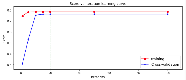
Analysis: with the increase of iteration, the score of logistic regression model is increasing. When the iteration exceeds 20, the score of the model is basically unchanged

6.1.2} change the size of data

# Chaning the sampling size
# set the iter to the best iteration: iter = 20

perc = [0.01,0.02,0.05,0.1,0.2,0.5,1]

kf = KFold(n_splits=3, random_state=RANDOM_STATE)

train_score = []
cv_score = []

# select a k:
k_ndcg = 5

for i, item in enumerate(perc):
    
    lr = LogisticRegression(C=1.0, max_iter=20, tol=1e-6, solver='newton-cg', multi_class='ovr')
    train_score_iter = []
    cv_score_iter = []
    
    n = int(xtrain_new.shape[0]*item)
    xtrain_perc = xtrain_new[:n, :]
    ytrain_perc = ytrain_new[:n]


    for train_index, test_index in kf.split(xtrain_perc, ytrain_perc):
        
        X_train, X_test = xtrain_perc[train_index, :], xtrain_perc[test_index, :]
        y_train, y_test = ytrain_perc[train_index], ytrain_perc[test_index]

        print(X_train.shape, X_test.shape)
        
        lr.fit(X_train, y_train)

        y_pred = lr.predict_proba(X_test)
        train_ndcg_score = ndcg_score(y_train, lr.predict_proba(X_train), k = k_ndcg)
        cv_ndcg_score = ndcg_score(y_test, y_pred, k=k_ndcg)

        train_score_iter.append(train_ndcg_score)
        cv_score_iter.append(cv_ndcg_score)
        
    train_score.append(np.mean(train_score_iter))
    cv_score.append(np.mean(cv_score_iter))
    

ymin = np.min(cv_score)-0.1
ymax = np.max(train_score)+0.1

plt.figure(figsize=(9,4))
plt.plot(np.array(perc)*100, train_score, 'ro-', label = 'training')
plt.plot(np.array(perc)*100, cv_score, 'bo-', label = 'Cross-validation')
plt.xlabel("Sample size (unit %)")
plt.ylabel("Score")
plt.xlim(-5, np.max(perc)*100+10)
plt.ylim(ymin, ymax)

plt.legend(loc = 'lower right', fontsize = 12)
plt.title("Score vs sample size learning curve")

plt.tight_layout()

 

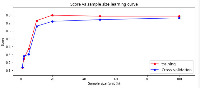
Analysis: with the increase of the amount of data, the prediction score (blue line) of the logistic regression model on the test set is rising, because we only use 10% of the data when training the model. If we use all the data, the effect may be better

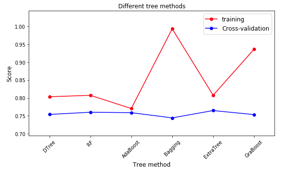
6.2 tree model

The models include DecisionTree, RandomForest, AdaBoost, Bagging, ExtraTree and GraBoost
 

from sklearn.ensemble import AdaBoostClassifier, BaggingClassifier, ExtraTreesClassifier
from sklearn.ensemble import GradientBoostingClassifier, RandomForestClassifier
from sklearn.tree import DecisionTreeClassifier
from sklearn.ensemble import *
from sklearn.svm import SVC, LinearSVC, NuSVC
LEARNING_RATE = 0.1
N_ESTIMATORS = 50
RANDOM_STATE = 2017
MAX_DEPTH = 9

#Built a tree dictionary
clf_tree ={
    'DTree': DecisionTreeClassifier(max_depth=MAX_DEPTH,
                                    random_state=RANDOM_STATE),
    
    'RF': RandomForestClassifier(n_estimators=N_ESTIMATORS,
                                 max_depth=MAX_DEPTH,
                                 random_state=RANDOM_STATE),
    
    'AdaBoost': AdaBoostClassifier(n_estimators=N_ESTIMATORS,
                                   learning_rate=LEARNING_RATE,
                                   random_state=RANDOM_STATE),
    
    'Bagging': BaggingClassifier(n_estimators=N_ESTIMATORS,
                                 random_state=RANDOM_STATE),
    
    'ExtraTree': ExtraTreesClassifier(max_depth=MAX_DEPTH,
                                      n_estimators=N_ESTIMATORS,
                                      random_state=RANDOM_STATE),
    
    'GraBoost': GradientBoostingClassifier(learning_rate=LEARNING_RATE,
                                           max_depth=MAX_DEPTH,
                                           n_estimators=N_ESTIMATORS,
                                           random_state=RANDOM_STATE)
}
train_score = []
cv_score = []

kf = KFold(n_splits=3, random_state=RANDOM_STATE)

k_ndcg = 5

for key in clf_tree.keys():
    
    clf = clf_tree.get(key)
    
    train_score_iter = []
    cv_score_iter = []

    for train_index, test_index in kf.split(xtrain_new, ytrain_new):

        X_train, X_test = xtrain_new[train_index, :], xtrain_new[test_index, :]
        y_train, y_test = ytrain_new[train_index], ytrain_new[test_index]
        
        clf.fit(X_train, y_train)

        y_pred = clf.predict_proba(X_test)
        train_ndcg_score = ndcg_score(y_train, clf.predict_proba(X_train), k = k_ndcg)
        cv_ndcg_score = ndcg_score(y_test, y_pred, k=k_ndcg)

        train_score_iter.append(train_ndcg_score)
        cv_score_iter.append(cv_ndcg_score)
        
    train_score.append(np.mean(train_score_iter))
    cv_score.append(np.mean(cv_score_iter))

train_score_tree = train_score
cv_score_tree = cv_score

ymin = np.min(cv_score)-0.05
ymax = np.max(train_score)+0.05

x_ticks = clf_tree.keys()

plt.figure(figsize=(8,5))
plt.plot(range(len(x_ticks)), train_score_tree, 'ro-', label = 'training')
plt.plot(range(len(x_ticks)),cv_score_tree, 'bo-', label = 'Cross-validation')

plt.xticks(range(len(x_ticks)),x_ticks,rotation = 45, fontsize = 10)
plt.xlabel("Tree method", fontsize = 12)
plt.ylabel("Score", fontsize = 12)
plt.xlim(-0.5, 5.5)
plt.ylim(ymin, ymax)

plt.legend(loc = 'best', fontsize = 12)
plt.title("Different tree methods")

plt.tight_layout()

 

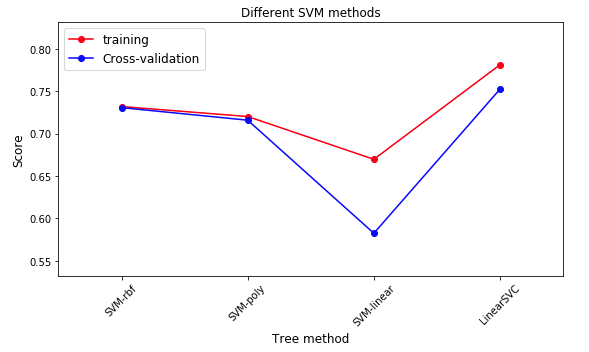
6.3 SVM model

• According to different kernel functions, it can be divided into SVM RBF, SVM poly, SVM linear, etc

TOL = 1e-4
MAX_ITER = 1000

clf_svm = {
    
    'SVM-rbf': SVC(kernel='rbf',
                   max_iter=MAX_ITER,
                   tol=TOL, random_state=RANDOM_STATE,
                   decision_function_shape='ovr'),     
    
    'SVM-poly': SVC(kernel='poly',
                   max_iter=MAX_ITER,
                   tol=TOL, random_state=RANDOM_STATE,
                   decision_function_shape='ovr'),     
    
    'SVM-linear': SVC(kernel='linear',
                      max_iter=MAX_ITER,
                      tol=TOL, 
                      random_state=RANDOM_STATE,
                      decision_function_shape='ovr'),  
    
    'LinearSVC': LinearSVC(max_iter=MAX_ITER,
                            tol=TOL,
                            random_state=RANDOM_STATE,
                            multi_class = 'ovr')  
                            
}     

train_score_svm = []
cv_score_svm = []

kf = KFold(n_splits=3, random_state=RANDOM_STATE)

k_ndcg = 5

for key in clf_svm.keys():
    
    clf = clf_svm.get(key)

    train_score_iter = []
    cv_score_iter = []

    for train_index, test_index in kf.split(xtrain_new, ytrain_new):

        X_train, X_test = xtrain_new[train_index, :], xtrain_new[test_index, :]
        y_train, y_test = ytrain_new[train_index], ytrain_new[test_index]
        
        clf.fit(X_train, y_train)

        y_pred = clf.decision_function(X_test)
        train_ndcg_score = ndcg_score(y_train, clf.decision_function(X_train), k = k_ndcg)
        cv_ndcg_score = ndcg_score(y_test, y_pred, k=k_ndcg)

        train_score_iter.append(train_ndcg_score)
        cv_score_iter.append(cv_ndcg_score)
        
    train_score_svm.append(np.mean(train_score_iter))
    cv_score_svm.append(np.mean(cv_score_iter))

ymin = np.min(cv_score_svm)-0.05
ymax = np.max(train_score_svm)+0.05

x_ticks = clf_svm.keys()

plt.figure(figsize=(8,5))
plt.plot(range(len(x_ticks)), train_score_svm, 'ro-', label = 'training')
plt.plot(range(len(x_ticks)),cv_score_svm, 'bo-', label = 'Cross-validation')

plt.xticks(range(len(x_ticks)),x_ticks,rotation = 45, fontsize = 10)
plt.xlabel("Tree method", fontsize = 12)
plt.ylabel("Score", fontsize = 12)
plt.xlim(-0.5, 3.5)
plt.ylim(ymin, ymax)

plt.legend(loc = 'best', fontsize = 12)
plt.title("Different SVM methods")

plt.tight_layout()

 

6.4 xgboost

• A model commonly used in kaggle competition

import xgboost as xgb

def customized_eval(preds, dtrain):
    labels = dtrain.get_label()
    top = []
    for i in range(preds.shape[0]):
        top.append(np.argsort(preds[i])[::-1][:5])
    mat = np.reshape(np.repeat(labels,np.shape(top)[1]) == np.array(top).ravel(),np.array(top).shape).astype(int)
    score = np.mean(np.sum(mat/np.log2(np.arange(2, mat.shape[1] + 2)),axis = 1))
    return 'ndcg5', score
# xgboost parameters

NUM_XGB = 200

params = {}
params['colsample_bytree'] = 0.6
params['max_depth'] = 6
params['subsample'] = 0.8
params['eta'] = 0.3
params['seed'] = RANDOM_STATE
params['num_class'] = 12
params['objective'] = 'multi:softprob'   # output the probability instead of class. 
train_score_iter = []
cv_score_iter = []

kf = KFold(n_splits = 3, random_state=RANDOM_STATE)

k_ndcg = 5

for train_index, test_index in kf.split(xtrain_new, ytrain_new):

    X_train, X_test = xtrain_new[train_index, :], xtrain_new[test_index, :]
    y_train, y_test = ytrain_new[train_index], ytrain_new[test_index]
    
    train_xgb = xgb.DMatrix(X_train, label= y_train)
    test_xgb = xgb.DMatrix(X_test, label = y_test)
    
    watchlist = [ (train_xgb,'train'), (test_xgb, 'test') ]

    bst = xgb.train(params, 
                     train_xgb,
                     NUM_XGB,
                     watchlist,
                     feval = customized_eval,
                     verbose_eval = 3,
                     early_stopping_rounds = 5)
    
    
    #bst = xgb.train( params, dtrain, num_round, evallist )

    y_pred = np.array(bst.predict(test_xgb))
    y_pred_train = np.array(bst.predict(train_xgb))
    train_ndcg_score = ndcg_score(y_train, y_pred_train , k = k_ndcg)
    cv_ndcg_score = ndcg_score(y_test, y_pred, k=k_ndcg)

    train_score_iter.append(train_ndcg_score)
    cv_score_iter.append(cv_ndcg_score)

train_score_xgb = np.mean(train_score_iter)
cv_score_xgb = np.mean(cv_score_iter)

print ("\nThe training score is: {}".format(train_score_xgb))
print ("The cv score is: {}\n".format(cv_score_xgb))

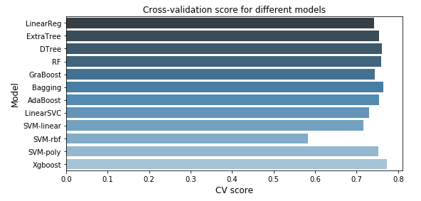
7. Model comparison

model_cvscore = np.hstack((cv_score_lr, cv_score_tree, cv_score_svm, cv_score_xgb))
model_name = np.array(['LinearReg','ExtraTree','DTree','RF','GraBoost','Bagging','AdaBoost','LinearSVC','SVM-linear','SVM-rbf','SVM-poly','Xgboost'])
fig = plt.figure(figsize=(8,4))

sns.barplot(model_cvscore, model_name, palette="Blues_d")

plt.xticks(rotation=0, size = 10)
plt.xlabel("CV score", fontsize = 12)
plt.ylabel("Model", fontsize = 12)
plt.title("Cross-validation score for different models")

plt.tight_layout()

 

8. Summary

1. Understanding and exploring data is very important
2. Features can be further extracted through feature engineering
3. There are many methods of model evaluation. Select the appropriate model evaluation method
4. At present, only 10% of the data is used for model training, and the effect may be better if all the data sets are used for training
5. We need to deeply study the model algorithm and learn to adjust parameters