We should be very familiar with expression chip data processing. We have a series of tweets,
It can basically cope with mainstream chip data, mainly affymetrix, illumina and agilent. Of course, the simplest is affymetrix chip, but recently many partners asked illumina chip data, mainly because some data output authors are not familiar with themselves, so they did not upload data according to the rules, As a result, we can't use standard code to deal with it.
For example, data in: https://www.ncbi.nlm.nih.gov/geo/query/acc.cgi?acc=GSE58539
You can see that there are two different forms of files on this page. The first contact partner may hesitate to download which one:
File type/resource
GSE58539_Non-normalized_data.txt.gz 4.8 Mb (ftp)(http) TXT
GSE58539_RAW.tar 26.2 Mb (http)(custom) TAR
It's actually GSE58539_Non-normalized_data.txt.gz This 4.8 Mb file is OK. Download it yourself.
The code for reading the expression matrix file normally is as follows:
library(GEOquery)
library(limma)
library(annotate)
library(lumi)
studyID='GSE58539'
fileName <- 'GSE58539_Non-normalized_data.txt' # Not Run
x.lumi <- lumiR.batch(fileName) ##, sampleInfoFile='sampleInfo.txt')
pData(phenoData(x.lumi))
## Do all the default preprocessing in one step
#lumi.N.Q <- lumiExpresso(x.lumi, normalize = F)
lumi.N.Q <- lumiExpresso(x.lumi)
### retrieve normalized data
dat <- exprs(lumi.N.Q)
dim(dat)#Look at the dimension of dat matrix
# GPL13667
dat[1:4,1:4] #Look at dat the 1 to 4 rows and 1 to 4 columns of this matrix. The row before the comma and the column after the comma
boxplot(dat[ ,1:4] ,las=2)

save(dat,file = 'dat_from_lumiR.batch.Rdata')
It can be seen that this is already a very normal chip expression matrix:
             5786057055_A 5786057055_B 5786057055_C 5786057055_D
ILMN_1343291    14.257948    14.120031    14.162906    14.188226
ILMN_1343295    12.500787    12.786823    13.043421    12.972077
ILMN_1651199     6.576717     6.544162     6.593763     6.503210
ILMN_1651209     6.684041     6.733616     6.713588     6.805869
Why don't we use the gse chip dataset processing code of the standard geo database? Let's see:
rm(list = ls())
options(stringsAsFactors = F)
f='GSE58539_eSet.Rdata'
# https://www.ncbi.nlm.nih.gov/geo/query/acc.cgi?acc=GSE58539
library(GEOquery)
# This package needs to pay attention to two configurations. Generally speaking, automatic configuration is sufficient.
#Setting options('download.file.method.GEOquery'='auto')
#Setting options('GEOquery.inmemory.gpl'=FALSE)
if(!file.exists(f)){
  gset <- getGEO('GSE58539', destdir=".",
                 AnnotGPL = F,     ## Annotate Document
                 getGPL = F)       ## Platform file
  save(gset,file=f)   ## Save to local
}
load('GSE58539_eSet.Rdata')  ## Load data
class(gset)  #View data type
length(gset)  #
class(gset[[1]])
gset

# Because this GEO dataset has only one GPL platform, what you download is a list containing one element
a=gset[[1]] #
dat=exprs(a) #Now we need to know that expa is an object through the description of this function
dim(dat)#Look at the dimension of dat matrix
# GPL13667
dat[1:4,1:4] #Look at dat the 1 to 4 rows and 1 to 4 columns of this matrix. The row before the comma and the column after the comma
boxplot(dat[ ,1:4] ,las=2)
colMeans(dat[ ,1:4])
save(dat,file = 'dat_from_GEOquery.Rdata')
It can be seen that the expression matrix at this time is actually zscore, as shown below:
> dat[1:4,1:4] #Look at dat the 1 to 4 rows and 1 to 4 columns of this matrix. The row before the comma and the column after the comma
              GSM1413151   GSM1413152 GSM1413153  GSM1413154
ILMN_1343291  0.09844685 -0.043561935 0.00000000  0.02590084
ILMN_1343295 -0.11312294  0.176450730 0.43721294  0.36480618
ILMN_1651199  0.03707123  0.004797936 0.05399847 -0.03390265
ILMN_1651209 -0.02612686  0.022301674 0.00283289  0.09231090
Compare the two matrices, and the code is as follows:
rm(list = ls())
options(stringsAsFactors = F)

library(GEOquery)
library(limma)
library(annotate)
library(lumi)

load(file = 'dat_from_GEOquery.Rdata')
dat_from_GEOquery = dat
load(file = 'dat_from_lumiR.batch.Rdata')
dat_from_lumiR.batch = dat

colnames(dat_from_lumiR.batch)
colnames(dat_from_GEOquery)

library(reshape2)
library(ggpubr)
library(patchwork)
df=melt(dat_from_lumiR.batch)
head(df)
ggboxplot(melt(dat_from_lumiR.batch),
          x = "Var2", y = "value", width = 0.8) +
ggboxplot(melt(dat_from_GEOquery),
          x = "Var2", y = "value", width = 0.8)
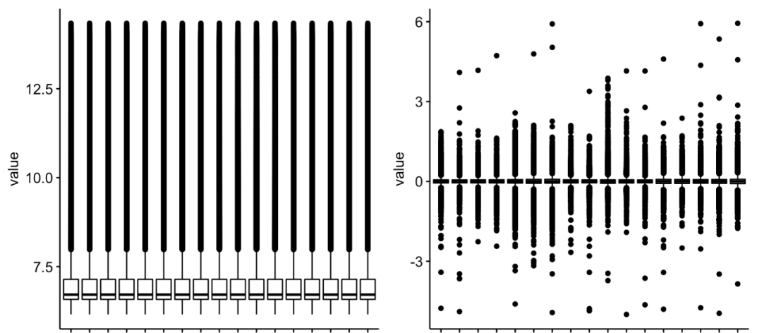
The diagram is as follows:

Compare the expression distribution of two expression matrices
It is also easy to see at this time that if the GSE chip data set processing code of the standard geo database gets the expression matrix by zscore, so it is generally not recommended to follow-up difference analysis, enrichment analysis and so on. But because the author gave GSE58539_Non-normalized_data.txt.gz This 4.8 Mb file is normal illumina chip data, and lumir of lumi package can be used After the batch function is read, the expression matrix capable of downstream analysis is obtained.
Ask a question: should all illumina chips be downloaded_ Non-normalized_data.txt.gz suffix file, go to the code I gave you above?
Apprenticeship assignment
For the two expression matrices, continue the subsequent difference analysis and enrichment analysis respectively, and compare the differences between the enrichment analysis results of the two subsequent difference analysis.
The results of the two difference analysis are presented by scatter diagram and Wayne diagram.
The results of two enrichment analyses are presented by gsea thermogram.
Write it at the end of the text
If you really think my tutorial is helpful to your scientific research project and makes you enlightened, or your project uses a lot of my skills, please add a short thank you when publishing your achievements in the future, as shown below:
We thank Dr.Jianming Zeng(University of Macau), and all the members of his bioinformatics team, biotrainee, for generously sharing their experience and codes.
If I have traveled around the world in universities and research institutes (including Chinese mainland) in ten years, I will give priority to seeing you if you have such a friendship.