In 2020, Vision Transformer based on self attention mechanism successfully applied the Transformer model used in NLP field to image classification in CV field, and obtained 88.55% accuracy on ImageNet data set.
However, there are two problems to be solved in order to truly apply the Transformer model to the whole CV field. 1. The problem of computational complexity caused by ultra-high resolution images; 2. There are many tasks in CV field, such as semantic segmentation, target detection, strength segmentation and other intensive prediction tasks. The original Vision Transformer did not have multi-scale prediction, so only one task can work well in classification.
Aiming at the first problem, by referring to the working mode of convolution network and window self attention model, swing transformer proposes a self attention model with moving window. Through the series window self attention operation (W-MSA) and sliding window self attention operation (SW-MSA), the swing transformer not only obtains the near global attention ability, but also reduces the amount of calculation from the square relationship of image size to linear relationship, which greatly reduces the amount of calculation and improves the speed of model reasoning.
To solve the second problem, in each module (Swin Transformer Block), Swin Transformer performs a down sampling after each feature extraction by means of feature fusion (PatchMerging, refer to the pooling operation in convolution network), which increases the receptive field of the next window attention operation on the original image, so as to carry out multi-scale feature extraction on the input image, The performance of other intensive predictive tasks in the CV field is also SOTA.
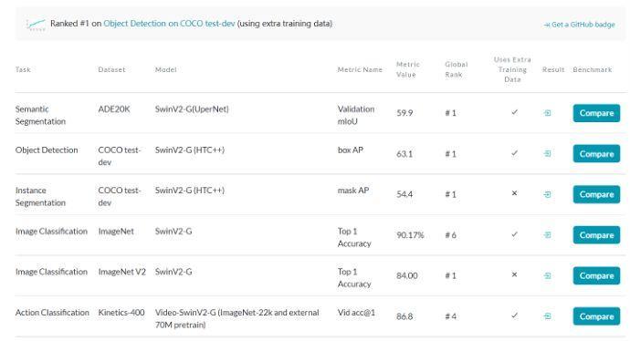
The following figure is a screenshot of paperwithcode. As of January 22, 2022, Swin Transformer is still dominant in various CV tasks. In the CV field, it's great to increase the accuracy by 1% on a certain task, while the swing transformer improves the accuracy by 2% ~ 3% on various tasks.
Turn the swing transformer core
Value of making SwinT modules
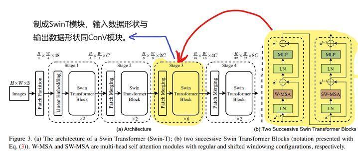
As shown in the figure below, the core module of Swin Transformer is the yellow part. We need to make this part into a general SwinT interface, so that more developers familiar with CNN can apply Swin Transformer to different tasks in the CV field.
The value of doing so has two points: 1. Swing transformer has strong capabilities, and this interface will not be outdated. ① The supercomputing unit required to realize the global attention calculation of a large-scale whole picture will not appear in a short time (it is difficult for individual developers to have this computing power), that is, the window attention can still be used for one to two years; ② Now it is generally believed that simple and effective is the best, while the implementation of swing transformer is very simple, which is easy for people to understand and remember its working principle; ③ In practice, swing transformer also won SOTA and successfully won the Mar award. The combination of simplicity and strength is the reason why it can win the Mar award.
2. Realize convenient and fast programming. For example, if we want to turn Unet into swin Unet, we just need to directly replace Conv2D module with SwinT module. We usually need to use not only the blocks in the Swin Transformer, but also the Conv2D module in the same network (for example, Swin Transformer is used to extract global features in the upper layer and Conv2D is used to extract local features in the lower layer). Therefore, we need to make architectural changes to the original Swin Transformer model.
Why can mobile window have the ability of global feature extraction
How the attention mechanism works in swing transformer is shown in the following figure. First, we perform self attention operation on the window in each color, such as [1,2,3,4], [5,6,7,8], [9,10,11,12], [13,14,15,16] and the elements in each list.
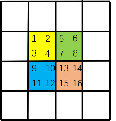
Then, the sliding window can be regarded as the re segmentation of the image by sliding the background black frame on the image.
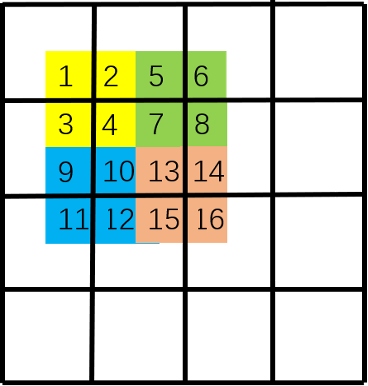
Finally, the image is restored to its original size. This step is convenient for code writing, and no attention operation is performed on the originally non adjacent areas in the window. Note that the window is determined by the black box. That is, because [4,7,10,13] in the original image are adjacent, the upper left corner [4,7,10,13] performs attention calculation together; Since [16,11,6,1] are not adjacent to each other, the lower right corner [16], [11], [6], [1] does attention calculation alone, while [16], [11] does not. The lower left corner [12,15] and [2,5] are adjacent to each other, so [12,15] does attention operation, [2,5] does attention operation, and there is no attention operation between [12,15] and [2,5].
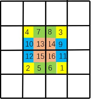
Through these two steps, wonderful things happened. In the first step, we established the connection between [1,2,3,4], [5,6,7,8], [9,10,11,12], [13,14,15,16] and then established the connection between [4,7,10,13] in the second step. It can be observed that through these two steps, we can establish the connection between [1,2,3,4,5,6,7,8,9,10,11,12]. The sliding window + original window is like a high-speed channel, establishing the connection of self attention between the upper left corner and the lower right corner of the image, so as to obtain the global receptive field.
We can find that sliding window and non sliding window are indispensable. Only when the two exist at the same time can we build global attention. Therefore, W-MSA and SW-MSA must be used together as a whole. Later, in the source code of our SwinT module, we will use W-MSA, SW-MSA and PatchMerging to sample, and integrate these three parts into one module. In the follow-up of this article, we will demonstrate how to use this interface to truly build a SwinResnet network and test its performance!
Usage of SwinT interface
For the source code of SwinT interface, please refer to:
https://aistudio.baidu.com/aistudio/projectdetail/3288357
#Import package. miziha contains SwinT module
import paddle
import paddle.nn as nn
import miziha

#Create test data
test_data = paddle.ones([2, 96, 224, 224]) #[N, C, H, W]
print(f'Enter size:{test_data.shape}')

#Create a SwinT layer
'''
Parameters:
in_channels: Number of input channels, same as convolution
out_channels: Number of output channels, same as convolution

The following is SwinT Unique, similar to the kernel size, stride, filling, etc. in convolution
input_resolution: Enter the size of the image
num_heads: The number of heads of multi head attention should be set to a value that can be divided by the number of input channels
window_size: The size of the window for attention calculation. The larger the window, the slower the operation will be
qkv_bias: qkv Offset, default None
qk_scale: qkv The scale, a normalization of attention size, defaults None      #Version V1 swin
dropout: default None
attention_dropout: default None
droppath: default None
downsample: Down sampling, default False,Set to True When, the size of the output picture will become half that of the input
'''
swint1 = miziha.SwinT(in_channels=96, out_channels=256, input_resolution=(224,224), num_heads=8, window_size=7, downsample=False)
swint2 = miziha.SwinT(in_channels=96, out_channels=256, input_resolution=(224,224), num_heads=8, window_size=7, downsample=True)
conv1 = nn.Conv2D(in_channels=96, out_channels=256, kernel_size=3, stride=1, padding=1)

#Forward propagation, printout shape
output1 = swint1(test_data)
output2 = swint2(test_data)
output3 = conv1(test_data)

print(f'SwinT Output size of:{output1.shape}')
print(f'Down sampled SwinT Output size of:{output2.shape}')  #Down sampling
print(f'Conv2D Output size of:{output3.shape}')
Run the above code and the model will output:
Enter size:[2, 96, 224, 224]
SwinT Output size of:[2, 256, 224, 224]
Down sampled SwinT Output size of:[2, 256, 112, 112]
Conv2D Output size of:[2, 256, 224, 224]
Replace Conv2D model in Resnet with SwinT
Create swing RESNET and test it!
In this part, we actually show how to use SwinT to replace the corresponding Conv2D module in the existing model. The whole process has little change to the source code.
Source code link:
https://www.paddlepaddle.org.cn/tutorials/projectdetail/3106582#anchor-10
In order to show the actual effect, we use Cifar10 data set (which is a data set with simple task and less data) to give the results of model accuracy and speed. It is proved that the effect of SwinT module is at least no worse than Conv2D. Since it takes 6 hours to run the whole process, there is no excessive adjustment of super parameters to prevent over fitting. Although the ordinary resnet50 can increase the batch to improve the speed, the batch size is a parameter related to the model regularization, so the batch is controlled at one size for comparison test.
First, create the convolution batch normalization block. The batchnorm is used in resnet50, and the layernorm is already included in the SwinT module, so this code does not need to be changed.
# ResNet model code
# BatchNorm layer is used in ResNet, and BatchNorm is added after the convolution layer to improve the numerical stability
# Define convolution batch normalization block
class ConvBNLayer(paddle.nn.Layer):
    def __init__(self,
                 num_channels,
                 num_filters,
                 filter_size,
                 stride=1,
                 groups=1,
                 act=None):


        # num_channels, number of input channels of convolution layer
        # num_filters, number of output channels of convolution layer
        # Stride, stride of convolution layer
        # Groups, the number of groups for grouping convolution. Default groups=1. Grouping convolution is not used

        super(ConvBNLayer, self).__init__()

        # Create a volume layer
        self._conv = nn.Conv2D(
            in_channels=num_channels,
            out_channels=num_filters,
            kernel_size=filter_size,
            stride=stride,
            padding=(filter_size - 1) // 2,
            groups=groups,
            bias_attr=False)

        # Create BatchNorm layer
        self._batch_norm = paddle.nn.BatchNorm2D(num_filters)

        self.act = act

    def forward(self, inputs):
        y = self._conv(inputs)
        y = self._batch_norm(y)
        if self.act == 'leaky':
            y = F.leaky_relu(x=y, negative_slope=0.1)
        elif self.act == 'relu':
            y = F.relu(x=y)
        return y
In this part, we define the residual block, which is the core unit of Resnet. We need to replace Conv2D with SwinT.
# Define residual block
# Each residual block will convolute the input picture three times, and then short circuit with the input picture
# If the shape of the third convolution output characteristic image in the residual block is inconsistent with the input, 1x1 convolution is performed on the input image to adjust its output shape to be consistent
class BottleneckBlock(paddle.nn.Layer):
    def __init__(self,
                 num_channels,
                 num_filters,
                 stride,
                 resolution,
                 num_heads=8,
                 window_size=8,
                 downsample=False,
                 shortcut=True):
        super(BottleneckBlock, self).__init__()
        # Create the first volume layer 1x1
        self.conv0 = ConvBNLayer(
            num_channels=num_channels,
            num_filters=num_filters,
            filter_size=1,
            act='relu')

        # Create a second convolution layer 3x3
        # self.conv1 = ConvBNLayer(
        #     num_channels=num_filters,
        #     num_filters=num_filters,
        #     filter_size=3,
        #     stride=stride,
        #     act='relu')

        #If the size is 7x7, start cnn, because it is not easy to divide equal size windows
        # Replace with SwinT as follows
        if resolution == (7,7):
            self.swin = ConvBNLayer(num_channels=num_filters,
                                    num_filters=num_filters,
                                    filter_size=3,
                                    stride=1,
                                    act='relu')
        else:
            self.swin = miziha.SwinT(in_channels=num_filters,
                                out_channels=num_filters,
                                input_resolution=resolution,
                                num_heads=num_heads,
                                window_size=window_size,
                                downsample=downsample)

        # Create a third convolution 1x1, but multiply the number of output channels by 4
        self.conv2 = ConvBNLayer(
            num_channels=num_filters,
            num_filters=num_filters * 4,
            filter_size=1,
            act=None)

        # If the output of conv2 is consistent with the input data shape of this residual block, then shortcut=True
        # Otherwise, shortcut = False, add a 1x1 convolution to the input data to make its shape consistent with conv2
        if not shortcut:
            self.short = ConvBNLayer(
                num_channels=num_channels,
                num_filters=num_filters * 4,
                filter_size=1,
                stride=stride)

        self.shortcut = shortcut

        self._num_channels_out = num_filters * 4

    def forward(self, inputs):

        y = self.conv0(inputs)
        swin = self.swin(y)
        conv2 = self.conv2(swin)

        # If shortcut=True, add the inputs directly to the output of conv2
        # Otherwise, the inputs need to be convoluted once to adjust the shape to be consistent with the conv2 output
        if self.shortcut:
            short = inputs
        else:
            short = self.short(inputs)

        y = paddle.add(x=short, y=conv2)
        y = F.relu(y)
        return y
Finally, we build a complete SwinResnet.
#Set up SwinResnet
class SwinResnet(paddle.nn.Layer):
    def __init__(self, num_classes=12):
        super().__init__()

        depth = [3, 4, 6, 3]
        # The number of convolution output channels used in the residual block, the size information of the picture, and the multi head attention parameters
        num_filters = [64, 128, 256, 512]
        resolution_list = [[(56,56),(56,56)],[(56,56),(28,28)],[(28,28),[14,14]],[(14,14),(7,7)]]
        num_head_list = [4, 8, 16, 32]

        # The first module of SwinResnet contains a 7x7 convolution followed by a maximum pooling layer
        #[3, 224, 224]
        self.conv = ConvBNLayer(
            num_channels=3,
            num_filters=64,
            filter_size=7,
            stride=2,
            act='relu')
        #[64, 112, 112]
        self.pool2d_max = nn.MaxPool2D(
            kernel_size=3,
            stride=2,
            padding=1)
        #[64, 56, 56]

        # The second to fifth modules c2, c3, c4 and c5 of SwinResnet
        self.bottleneck_block_list = []
        num_channels = 64
        for block in range(len(depth)):
            shortcut = False
            for i in range(depth[block]):
                # c3, c4 and c5 will use downsample=True in the first residual block; All other residual blocks downsample=False
                bottleneck_block = self.add_sublayer(
                    'bb_%d_%d' % (block, i),
                    BottleneckBlock(
                        num_channels=num_channels,
                        num_filters=num_filters[block],
                        stride=2 if i == 0 and block != 0 else 1,
                        downsample=True if i == 0 and block != 0 else False,
                        num_heads=num_head_list[block],
                        resolution=resolution_list[block][0] if i == 0 and block != 0 else resolution_list[block][1],
                        window_size=7,
                        shortcut=shortcut))
                num_channels = bottleneck_block._num_channels_out
                self.bottleneck_block_list.append(bottleneck_block)
                shortcut = True

        # Using global pooling on the output characteristic graph of c5
        self.pool2d_avg = paddle.nn.AdaptiveAvgPool2D(output_size=1)

        # stdv is used as the variance of random initialization parameters of the whole connection layer
        import math
        stdv1 = 1.0 / math.sqrt(2048 * 1.0)
        stdv2 = 1.0 / math.sqrt(256 * 1.0)

        # Create a full connection layer, and the output size is the number of categories. After convolution and global pooling of residual network,
        # The dimension of convolution feature is [B,2048,1,1], so the input dimension of the last layer of full connection is 2048
        self.out = nn.Sequential(nn.Dropout(0.2),
                        nn.Linear(in_features=2048, out_features=256,
                      weight_attr=paddle.ParamAttr(
                          initializer=paddle.nn.initializer.Uniform(-stdv1, stdv1))),
                        nn.LayerNorm(256),
                        nn.Dropout(0.2),
                        nn.LeakyReLU(),
                        nn.Linear(in_features=256,out_features=num_classes,
                        weight_attr=paddle.ParamAttr(
                          initializer=paddle.nn.initializer.Uniform(-stdv2, stdv2)))
                          )

    def forward(self, inputs):
        y = self.conv(inputs)
        y = self.pool2d_max(y)
        for bottleneck_block in self.bottleneck_block_list:
            y = bottleneck_block(y)
        y = self.pool2d_avg(y)
        y = paddle.reshape(y, [y.shape[0], -1])
        y = self.out(y)
        return y
Use the built network to train the model
Mode = 0    #Modify here to train three different models

import paddle
import paddle.nn as nn
from paddle.vision.models import resnet50, vgg16, LeNet
from paddle.vision.datasets import Cifar10
from paddle.optimizer import Momentum
from paddle.regularizer import L2Decay
from paddle.nn import CrossEntropyLoss
from paddle.metric import Accuracy
from paddle.vision.transforms import Transpose, Resize, Compose
from model import SwinResnet

# Make sure that from the pad vision. datasets. The image data loaded in cifar10 is NP Ndarray type
paddle.vision.set_image_backend('cv2')

# Loading model
resnet = resnet50(pretrained=False, num_classes=10)
import math
stdv1 = 1.0 / math.sqrt(2048 * 1.0)
stdv2 = 1.0 / math.sqrt(256 * 1.0)
#Modify the last layer of resnet to strengthen the ability of model fitting
resnet.fc = nn.Sequential(nn.Dropout(0.2),
                nn.Linear(in_features=2048, out_features=256,
                weight_attr=paddle.ParamAttr(
                    initializer=paddle.nn.initializer.Uniform(-stdv1, stdv1))),
                nn.LayerNorm(256),
                nn.Dropout(0.2),
                nn.LeakyReLU(),
                nn.Linear(in_features=256,out_features=10,
                weight_attr=paddle.ParamAttr(
                    initializer=paddle.nn.initializer.Uniform(-stdv2, stdv2)))
                    )
model = SwinResnet(num_classes=10) if Mode == 0 else resnet

#Packaging Model
model = paddle.Model(model)

# Create image transform
transforms = Compose([Resize((224,224)), Transpose()]) if Mode != 2 else Compose([Resize((32, 32)), Transpose()])

# Using the Cifar10 dataset
train_dataset = Cifar10(mode='train', transform=transforms)
valid_dadaset = Cifar10(mode='test', transform=transforms)

# Define optimizer
optimizer = Momentum(learning_rate=0.01,
                     momentum=0.9,
                     weight_decay=L2Decay(1e-4),
                     parameters=model.parameters())

# Prepare for training
model.prepare(optimizer, CrossEntropyLoss(), Accuracy(topk=(1, 5)))

# Start training
model.fit(train_dataset,
          valid_dadaset,
          epochs=40,
          batch_size=80,
          save_dir="./output",
          num_workers=8)
Analysis of test results
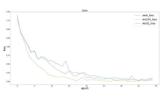
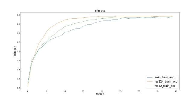
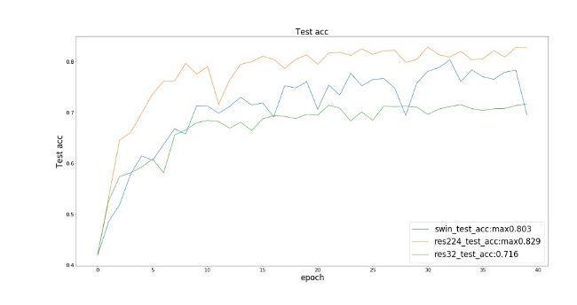
The following res224 refers to the Resnet50 input image size of 224x224, and res32 refers to the Resnet50 input image size of 32x32.
We observed that the three models (SwinResnet, res224 and res32) achieved similar results in training loss and training set accuracy; In terms of test accuracy, SwinResnet accuracy reaches 80.3%, res224 accuracy reaches 82.9%, and res32 accuracy reaches 71.6%. ① In terms of accuracy, there is little difference between SwinResnet and res224. Because this is a small data set, the ability of SwinResnet is actually limited, and the overall accuracy of SwinResnet is almost a linear improvement. ② In fact, the speed of a net batch operation is four times that of a net batch operation, which is 224 Ms.
On the other hand, we also found that the image size of Cifar10 dataset is actually 32x32, but the accuracy of interpolating it to 224 and then connecting Resnet is 11.3% higher than that of directly connecting Resnet. This is a huge improvement, although we have not introduced any additional amount of information. One explanation is: because Resnet is used to classify Imagenet pictures, and the image size is 224x224, it is not suitable for 32x32 pictures as the input of the model, although there is no difference in the amount of information between the two pictures. This reveals an inadaptability of the size change of convolution kernel, which is difficult to capture the information of objects with different sizes, which is caused by the fixed size of convolution kernel.
Application scenarios of SwinT
1. Use SwinT module to build a complete Swin Transformer model to reproduce the paper.
2. The existing Conv2D model can be replaced by SwinT to build a network with better performance, such as swin UNET, and where many layers of CNN need to be superimposed to extract depth features in various scenes, several Conv2D layers can be replaced with one SwinT. > 3. Because the input and output of SwinT are exactly the same as Conv2D, it can also be used in complex tasks such as semantic segmentation and target detection. > 4. SwinT and Conv2D can be used for model building at the same time. SwinT can be used when advanced global features need to be extracted and Conv2D can be used when local information is needed, which is very flexible.
summary
We have made the core module of Swin Transformer into a SwinT interface, which is similar to Conv2D. Firstly, it is very convenient for developers to write network models, especially when they want to customize the model architecture, and use Conv2D and SwinT together; Then, we think that the content of SwinT interface is very simple and efficient, so this interface will not be outdated in the short term, and can have the guarantee of timeliness; Finally, we test the interface in reality, and prove the ease of use and precision performance of the interface.
Project link: https://aistudio.baidu.com/aist