Today, let's share how matlab achieves an ant colony optimization algorithm to solve the traveler problem.
Ant Colony Optimization (ACO) algorithm is described in detail in the last blog post. A little buddy who needs it can see it
https://blog.csdn.net/HuangChen666/article/details/115827732
1. Initialize city information
1.1 Random city coordinates
1.2 Find the distance between cities
2. Initialization parameters
3. Iterate to find the best path
3.1 Randomly Generate Ant Start Cities
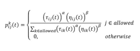
3.2 Iterative Calculation of Selected City Probability
3.3 roulette to pick the next city
3.4 Update Shortest Path
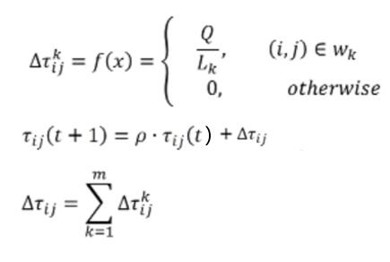
3.5 Update Pheromones
4. Result
5. All Codes
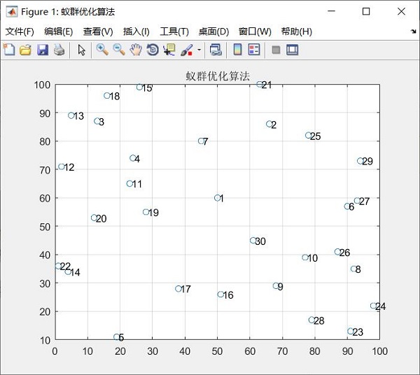
1. Initialize city information
1.1 Random city coordinates
1.2 Find the distance between cities
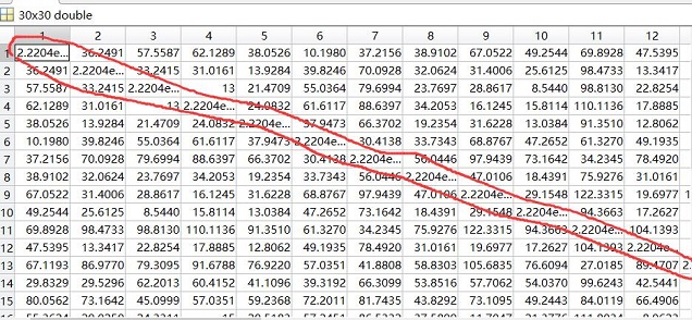
The diagonal line is the distance from city I to i, replaced by a small number.
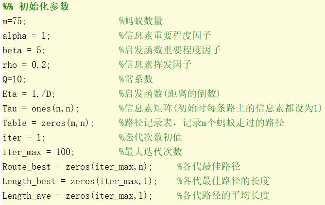
2. Initialization parameters
3. Iterate to find the best path
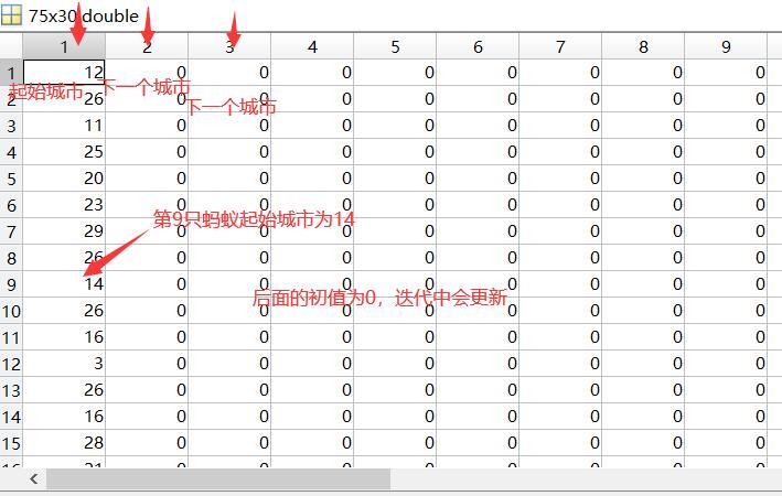
3.1 Randomly Generate Ant Start Cities
3.2 Iterative Calculation of Selected City Probability
3.3 roulette to pick the next city
https://blog.csdn.net/xuxinrk/article/details/80158786
3.4 Update Shortest Path
***It is important to note that the calculated shortest path for this time is not necessarily smaller than the last one, and the convergence trajectory of the resulting shortest path will fluctuate significantly, such as the following
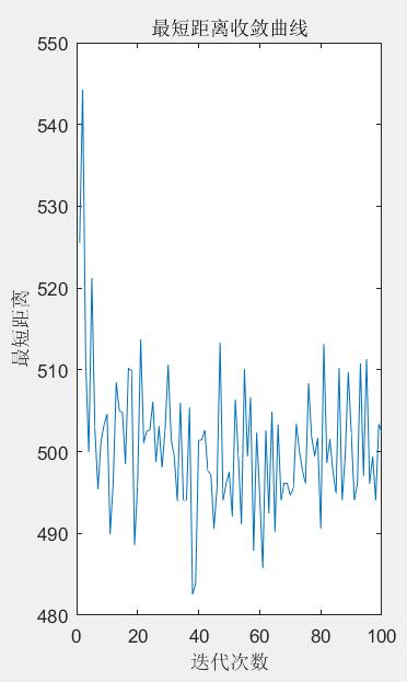
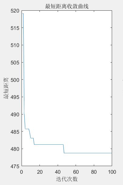
So here we can improve it, the basic idea is: if the shortest path size in this tour is larger than the last one, then the shortest path size in this tour will be changed to the same as the last one, so that there will be no shortest distance in the later iteration than the previous one, so the treatment will be more in line with people's ideas, more reasonable, and modified as follows
3.5 Update Pheromones
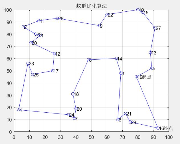
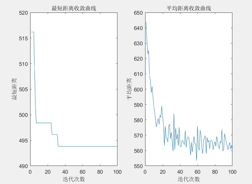
4. Result
Below are the shortest and average distance convergence curves
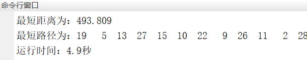
Command Line Output Results
5. All Codes
https://www.bilibili.com/video/BV1c4411W7zc
https://www.bilibili.com/video/BV1Z7411H78S?from=search&seid=14512389210209190890
clc;clear;
t0=clock; %For timing
%% Initialize city information
n=30; %Define the number of cities
city=[(randperm(100,n))',(randperm(100,n))']; %Getting city coordinates
figure('name','aco');
plot(city(:,1),city(:,2),'o'); %Tracing
for i=1:n
text(city(i,1)+0.5,city(i,2),num2str(i)); %Grade
end
title('aco');
%Set the range of the horizontal and vertical coordinates
grid on %Gridlines
hold on
%% Find the distance between cities
D=zeros(n,n); %Create a new one n*n Matrix storage distance of
for i=1:n
for j=1:n
if i~=j
D(i,j)=sqrt(sum((city(i,:)-city(j,:)).^2));
else
D(i,j)=eps; %Set to a small number, but not 0, as used in the following denominator
end
end
end
%% Initialization parameters
m=75; %Ant number
alpha = 1; %Pheromone Importance Factor
beta = 5; %Heuristic Importance Factor
rho = 0.2; %Pheromone Volatile Factor
Q=10; %constant coefficient
Eta = 1./D; %Heuristics(inverse distance)
Tau = ones(n,n); %Pheromone Matrix(Initially, each road's pheromone is set to 1)
Table = zeros(m,n); %Path Record Table, Record m Path taken by ants
iter = 1; %Initial value of iteration number
iter_max = 100; %Maximum number of iterations
Route_best = zeros(iter_max,n); %Best Routes for Generations
Length_best = zeros(iter_max,1); %Length of the best path for each generation
Length_ave = zeros(iter_max,1); %Average length of each generation path
%% Iterate to find the best path
for iter=1:iter_max
%Starting City for Random Ants
for i=1:m
Table(i,1)=randperm(n,1);
end
citys_index=1:n; %Define all city indexes
for i=1:m %Traverse all ants
for j=2:n %Traverse all other cities
tabu=Table(i,1:(j-1)); %Visited City(Prohibit access to tables)
allow=citys_index(~ismember(citys_index,tabu)); %Remove Visited Cities(City to visit)
P=allow; %Store probability, defined as anything, as long as and allow Same length
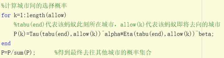
%Calculating the probability of selection between cities
for k=1:length(allow)
%tabu(end)Represents the city where the ant is now located. allow(k)The city where the ant is going
P(k)=Tau(tabu(end),allow(k))^alpha*Eta(tabu(end),allow(k))^beta;
end
P=P/sum(P); %Find the set of probabilities for ultimately going to another city
Pc=cumsum(P); %Cumulative probability
%Roulette Select Next City
target_index=find(Pc>=rand); %Find cases larger than random values from cumulative probability
target=allow(target_index(1)); %Take out the first result of the roulette
Table(i,j)=target; %Determine the i The first day an ant goes j-1 City
end
end
%Calculate the length of each ant's path once each ant has traveled
Length=zeros(m,1);
for i=1:m
for j=1:(n-1)
Length(i)=Length(i)+D(Table(i,j),Table(i,j+1));
end
%Last plus the distance from the last point to the starting point
Length(i)=Length(i)+D(Table(i,n),Table(i,1));
end
%% Calculating Shortest Path Distance and Average Distance
[min_length,min_index]=min(Length); %Take out the shortest path and its subscript
if iter==1
Length_best(iter)=min_length; %Save this shortest path distance
else
Length_best(iter)=min(Length_best(iter-1),min_length); %Select the shortest path that is smaller this time and last time
end
Route_best(iter,:)=Table(min_index,:); %Save this shortest route
Length_ave(iter)=mean(Length); %Save the average distance for this route
%% Update pheromone
Tau_Ant=Q./Length; %Pheromone concentration left by each ant along the path
Tau_Temp=zeros(n,n);
for i=1:m
for j=1:n-1
%Update pheromone
Tau_Temp(Table(i,j),Table(i,j+1))=Tau_Temp(Table(i,j),Table(i,j+1))+Tau_Ant(i);
end
%Update last node to start pheromone
Tau_Temp(Table(i,n),Table(i,1))=Tau_Temp(Table(i,n),Table(i,1))+Tau_Ant(i);
end
Tau=(1-rho)*Tau+Tau_Temp; %Adding new pheromones after evaporation of pheromones
Table = zeros(m,n); %Clear the route for the next round
end
%% Command Line Window Displays Results
[min_length,min_index]=min(Length_best); %Take out the shortest path and its subscript
Finnly_Route=Route_best(min_index,:);
last_time=etime(clock,t0);
disp(['The shortest distance is:' num2str(min_length)]);
disp(['The shortest path is:' num2str(Finnly_Route)]);
disp(['Runtime:' num2str(last_time) 'second']);
%% Mapping
plot([city(Finnly_Route,1);city(Finnly_Route,1)],...
[city(Finnly_Route,2);city(Finnly_Route,2)],'bo-'); %Tracing
text(city(Finnly_Route(1),1),city(Finnly_Route(1),2),' Starting point');
text(city(Finnly_Route(end),1),city(Finnly_Route(end),2),' End');
figure(2);
subplot(1,2,1); %First column displayed in one row and two columns of images
plot(Length_best);
xlabel('Number of iterations');
ylabel('Minimum distance');
title('Shortest distance convergence curve');
subplot(1,2,2); %The second column displayed in one row and two columns of images
plot(Length_ave);
xlabel('Number of iterations');
ylabel('Average Distance');
title('Average Distance Convergence Curve');