1, Introduction
Vector quantization is defined as the process of encoding points in a vector space with a finite subset. In vector quantization coding, the key is the establishment of codebook and codeword search algorithm. For example, the common clustering algorithm is a vector quantization method. In the ANN approximate nearest neighbor search, product quantization (PQ) is the most typical vector quantization method. At the end of the previous blog post on content-based image retrieval technology, the PQ product quantization method is briefly summarized. In this section, Pakchoi makes a more intuitive explanation of PQ product quantization and inverted product quantization (IVFPQ) in combination with the papers and codes he has read.
1 PQ product quantization
The core idea of PQ product quantization is clustering, or specifically applied to ANN approximate nearest neighbor search. K-Means is a special case where the number of PQ product quantization subspaces is 1. The process of generating codebook and quantization by PQ product quantization can be illustrated as follows: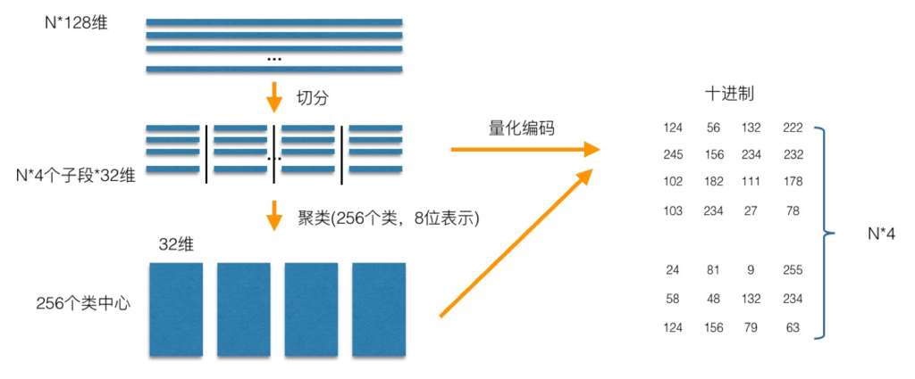
In the training phase, for N training samples, assuming that the sample dimension is 128 dimensions, we divide them into 4 subspaces, and the dimension of each subspace is 32 dimensions. Then, in each subspace, we use K-Means to cluster the subspaces (256 classes are schematically clustered in the figure), so that each subspace can get a codebook. In this way, each sub segment of the training sample can be approximated by the cluster center of the subspace, and the corresponding code is the ID of the class center. As shown in the figure, only one coding method is used to achieve the purpose of quantization, as shown in the figure. For the samples to be encoded, the same segmentation is performed, and then the nearest class center is found one by one in each subspace, and then they are represented by the ID of the class center, that is, the coding of the samples to be encoded is completed.
As mentioned above, in vector quantization coding, the key is the establishment of codebook and codeword search algorithm. Above, we get the established codebook and the way of quantization coding. The remaining focus is how to calculate the distance between the query sample and the sample in the dataset.
In the query stage, PQ is also calculating the distance between the query sample and each sample in the dataset, but the calculation of this distance is transformed into an indirect approximation method. When PQ product quantization method calculates distance, there are two distance calculation methods, one is symmetric distance, the other is asymmetric distance. The loss of asymmetric distance is small (that is, it is closer to the real distance), and this distance calculation method is often used in practice. The following process illustrates the calculation of the asymmetric distance (the part marked by the red box) between the query samples and the dataset samples when the query samples arrive: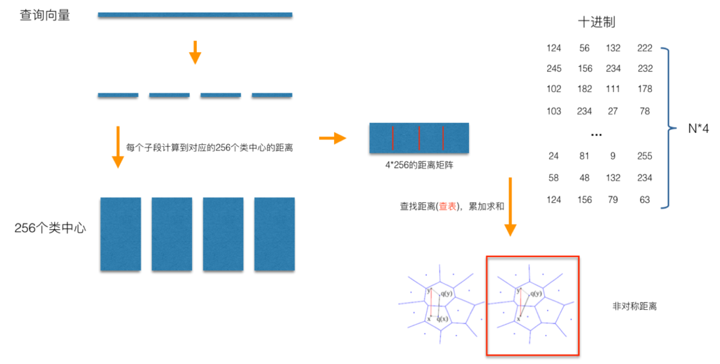
As shown in the figure, the distance of each sub segment in the training pool can be divided into four sub segments, and then it is easy to calculate the distance from each sub segment to the center of the training pool, as shown in the figure. When calculating the distance between a sample in the library and the query vector, such as the distance between the sample coded as (124, 56, 132, 222) and the query vector, we can take the corresponding distance of each sub segment from the distance pool. For example, for the sub segment coded as 124, we can take the distance numbered 124 out of the 256 distances calculated in the first, After the distances corresponding to all sub segments are taken out, the distances of these sub segments are summed to obtain the asymmetric distance between the sample and the query sample. After all the distances are calculated and sorted, we can get the final result we want.
From the above process, we can clearly see the principle that PQ product quantization can accelerate the index: that is, the distance calculation of the whole sample is transformed into the distance calculation to the center of the subspace class. For example, in the example above, the number of times to calculate the distance in the original brute force search method increases linearly with the number of samples N, but after PQ coding, for the time-consuming distance calculation, as long as it is calculated 4 * 256 times, the consumption of this time can be almost ignored. In addition, it can be seen from the above figure that after encoding the features, a relatively short encoding can be used to represent the samples, which naturally consumes much less memory than brute force search.
On some special occasions, we always want to obtain the exact distance rather than the approximate distance, and we always like to obtain the cosine similarity between vectors (the cosine similarity distance range is between [- 1,1], which is convenient to set a fixed threshold). For this scenario, we can quantify the front value obtained by PQ product top@K Make a sort of brute force search.
2 inverted product quantization
Inverted PQ product quantization (IVFPQ) is a further accelerated version of PQ product quantization. The essence of acceleration is inseparable from Chinese cabbage. The first emphasis is on the acceleration principle: brute force search is to search in the whole space. In order to speed up the search speed, almost all ANN methods divide the whole space into many small subspaces, and quickly lock in one (several) subspaces in some way during the search, Then do traversal in the (several) subspaces. As can be seen from the previous section, although the distance has been calculated in advance when PQ product quantifies the distance, for the distance from each sample to the query sample, we still have to sum and calculate the distance one by one. However, in fact, we are interested in those samples that are similar to the query samples (cabbage calls such areas of interest), that is, adding them honestly one by one actually does a lot of useless work. If we can quickly lock the global traversal into the area of interest by some means, we can omit unnecessary global calculation and sorting. The "inverted" of inverted PQ product quantization is the embodiment of such an idea. In the specific implementation means, clustering is used to realize the rapid positioning of the region of interest. In the inverted PQ product quantization, clustering can be said to be applied incisively and vividly.
The whole process of inverted PQ product quantization is shown in the figure below: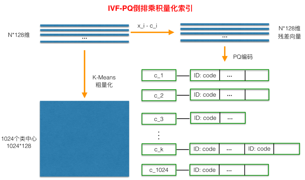
Before PQ product quantization, a rough quantization process is added. Specifically, K-Means is used to cluster N training samples. The number of clusters here should not be too large, which is generally set to 1024. This can complete the clustering process at a relatively fast speed. After getting the cluster center, for each sample X_ i. Find the nearest class center C_ After I, the two are subtracted to obtain sample X_ The residual vector (x_i-c_i) of I is the PQ product quantization process for (x_i-c_i), which will not be repeated.
When querying, through the same rough quantization, we can quickly locate which C the query vector belongs to_ I (i.e. in which region of interest), and then calculate the distance in the region of interest according to the PQ product quantization distance calculation method described above.
2, Source code
function mfc=my_mfcc(x,fs)
%MY_MFCC:obtain Speaker recognition Parameters of
%x:Input voice signal  fs: sampling rate
%mfc: dozen mfcc There are 36 parameters including coefficient, one energy and first-order and second-order difference, and one frame of data for each behavior
%clc,clear
%[x,fs]=audioread('wo6.wav');
N=256;p=24;
bank=mel_banks(p,N,fs,0,fs/2);
% normalization mel Filter bank coefficient
bank=full(bank);
bank=bank/max(bank(:));

% Normalized cepstrum lifting window
w = 1 + 6 * sin(pi * [1:12] ./ 12);
w = w/max(w);

% Pre emphasis filter
x=double(x);
x=filter([1 -0.9375],1,x);

% Speech signal framing
sf=check_ter(x,N,128,10);

x=div_frame(x,N,128);
%sf=sp_ter(x,4,16);
%m=zeros(size(x,1),13);
m=zeros(1,13);
% Calculation per frame MFCC parameter
for i=1:size(x,1)
    if sf(i)==1
        % j=j+1;
         y = x(i,:);
         y = y' .* hamming(N);
         energy=log(sum(y.^2)+eps);%energy
         y = abs(fft(y));
         y = y.^2+eps;
        c1=dct(log(bank * y));
        c2 = c1(2:13).*w';%Take 2~13 Coefficient
        %m(i,:)=[c2;energy]';
        m1=[c2;energy]';
        %m1=c2';
        m=[m;m1];
    end

end

%Difference coefficient
dm = zeros(size(m));
dmm= zeros(size(m));
for i=2:size(m,1)-1
  dm(i,:) = (m(i,:) - m(i-1,:));
end
for i=3:size(m,1)-2
  dmm(i,:) = (dm(i,:) - dm(i-1,:));
end
%dm = dm / 3;
function v=lbg(x,k)
%lbg: complete lbg Mean clustering algorithm
% lbg(x,k) For input samples x,Divide k Class. Among them, x by row*col Matrix, each column is a sample,
% Each sample has row Elements.
% [v1 v2 v3 ...vk]=lbg(...)return k Categories, of which vi Is a structure, vi.num For this class
% Number of elements contained in, vi.ele(i)For the first i Element values, vi.mea Is the average value of the corresponding category

[row,col]=size(x);
%u=zeros(row,k);%Each column is a central value
epision=0.03;%choice epision parameter
delta=0.01;
%u2=zeros(row,k);
%LBG Algorithm generation k Center
u=mean(x,2);%The first cluster center is the overall mean
for i3=1:log2(k)
    u=[u*(1-epision),u*(1+epision)];%double
    %time=0;
    D=0;
    DD=1;
    while abs(D-DD)/DD>delta   %sum(abs(u2(:).^2-u(:).^2))>0.5&&(time<=80)   %u2~=u
        DD=D;
        for i=1:2^i3            %initialization
            v(i).num=0;
            v(i).ele=zeros(row,1);
        end
        for i=1:col %The first i Samples
            distance=dis(u,x(:,i));%The first i Distance from each sample to each center
            [val,pos]=min(distance);
             v(pos).num=v(pos).num+1;%Number of elements plus 1
            if v(pos).num==1    %ele Empty
                v(pos).ele=x(:,i);
            else
                v(pos).ele=[v(pos).ele,x(:,i)];
            end
        end
        for i=1:2^i3
            u(:,i)=mean(v(i).ele,2);%New mean center
            for m=1:size(v(i).ele,2)
                D=D+sum((v(i).ele(m)-u(:,i)).^2);
            end
        end
    end
end
3, Operation results
4, Remarks
Complete code or write on behalf of QQ1575304183