1 Introduction
1.1 TSP introduction
"Traveling salesman problem" (TSP) can be simply described as: a seller starts from one of the n cities, does not repeatedly complete the other n-1 cities and returns to the original starting point, and finds the shortest path among all possible paths.
The route of a traveler can be regarded as a ring designed for n cities, or an arrangement of n cities in a row. Because the number of all possible traversals of n cities can reach (n-1)! Therefore, solving this problem requires O(n!) Calculation time of. The genetic algorithm developed by Professor Holland has become an efficient method to solve the global optimization problem.
1.2 solving tsp model by genetic algorithm
Traveling salesman problem (TSP) is a combinatorial optimization problem, which has become a standard problem to test new combinatorial optimization algorithms. Genetic algorithm is applied to solve TSP problem. Firstly, the sequence of visited cities is coded by permutation and combination, which ensures that each city passes through and only once. Then the initial population is generated and the fitness function is calculated, that is, the distance traversing all cities is calculated. Then the optimal preservation method is used to determine the selection operator to ensure that the excellent individuals can be copied directly to the next generation. The ordered crossover and inverted mutation methods are used to determine the crossover operator and mutation operator.
Algorithm flow
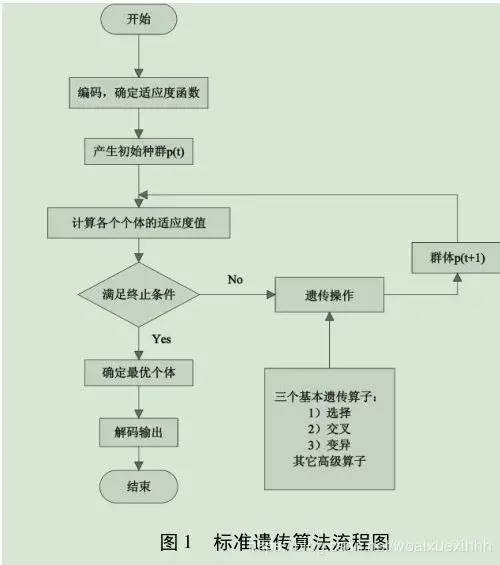
Genetic algorithm implementation of traveling salesman problem
1. Initial group setting
Generally, an initial population with scale n is randomly generated. Here, we define a pop matrix of s rows and t columns to represent the population. T is the number of cities + 1, that is, N + 1, and S is the number of individuals in the sample. In this paper, the TSP problem of 30 cities is discussed. At this time, the value of T is 31. The first 30 elements of each row in the matrix represent the number of cities passing through, and the last element represents the value of fitness function, that is, the distance sought by each individual.
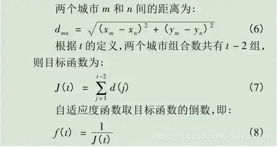
2. The design of fitness function is an evaluation function to judge its advantages and disadvantages according to individual fitness value. In this problem, the sum of distances is used as the fitness function to measure whether the solution result is optimal.
3. Selection refers to the operation of selecting the winning individual from the group with a certain probability. It is based on the evaluation of individual fitness in the group. In order to speed up the local search, the method of optimal preservation strategy is adopted in the algorithm, that is, the individual with the largest fitness in the group directly replaces the individual with the smallest fitness. They do not perform crossover and mutation operations, but directly copy to the next generation, so as not to destroy the excellent solutions in the population.
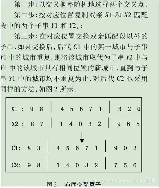
4. Crossover operator is the main means to generate new individuals. It refers to the operation of pairing individuals in pairs, replacing and reorganizing some structures of paired parent individuals with crossover probability Pc to generate new individuals. In this paper, the ordered crossover method is used. The steps of the ordered crossover method are described as follows:
5. Mutation operation is to change a bit or some bits on the individual coding string in the population with a small probability Pm, so as to generate a new individual. In this paper, the inverted mutation method is adopted: assuming that the current individual x is (1 374 805 962), if the current random probability value is less than Pm, two points mutatepoint(1) and mutatepoint(2) from the same individual are randomly selected, and then the middle part of the two points is inverted to produce a new individual. For example, suppose that two points "7" and "9" of individual X are randomly selected, the middle part of the two points is inverted, that is, "4805" becomes "5084", and a new individual x is (1 3 7 5 0 8 4 9 6 2).
6. The termination condition is a certain algebra of the cycle.
Part 2 code
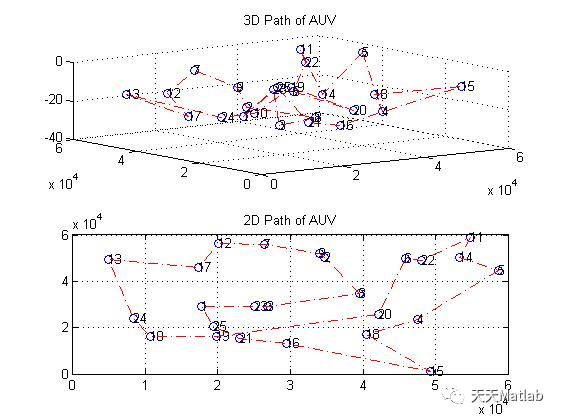
%%%%%%%%%% AUV path planning using GA %%%%%%%%%%%%%%%Run 'RP_coordinate.m' before running main %%%%clear all;close all;tic;%Runtime timer%% global variablesload ('coor.mat'); %Load data generated by RP_coordinate.mPopsize =50; %Population size, should be an even integer%Genetic parameters%MIXRATE = 0.3;ITERATION = 10000; %Number of iterationTHRESHOLD = 100;Pcross = 0.7; %Crossover ratePmutation = 0.3; %Mutation rate%BeginParentpop=InitPop(Popsize,RPNUM,adjacency);Fitnesscurve=[];Generation = 1; Fitconst=0; %Number of generations that fitness values remain constant%% Genetic algorithmwhile(Generation <= ITERATION) if (Fitconst<=THRESHOLD) %Stop iteration if fitness value is constant in threshold number of genreations fitness = Fitness(Parentpop,adjacency); %Calculate fitness of parents crossover = Crossover(Parentpop,Pcross); %Crossover Childpop = Mutation(crossover,Pmutation); %Mutate and get chindren combopop=[Parentpop;Childpop]; %Combine parents and chindren combofitness=Fitness(combopop,adjacency); %Calculate overall fitness nextpop=Select(combopop,combofitness); %Select the first half of best to get 2nd gen Parentpop=nextpop.pop; if(Generation ==1) Best_GApath=Parentpop(1,:); Best_Fitness=combofitness(nextpop.bestplan); else New_Best_Fitness=combofitness(nextpop.bestplan);%Evaluate best solution New_Best_GApath=Parentpop(1,:); if(New_Best_Fitness<Best_Fitness) Best_Fitness=New_Best_Fitness; Best_GApath=New_Best_GApath; Fitconst = 0; %%%%%%%%Visualize planning process%%%%%%%%% GENERATION=[1:Generation-1];% GAplancoor = [RP(Best_GApath).x;RP(Best_GApath).y; RP(Best_GApath).z].';% figure(1);% for i=1:RPNUM% subplot(2,1,1); %Plot all rendezvous points% plot3(RP(i).x,RP(i).y,RP(i).z,'o');% text(RP(i).x,RP(i).y, RP(i).z,num2str(i));% hold on;% subplot(2,1,2);% plot(RP(i).x,RP(i).y,'o');% text(RP(i).x,RP(i).y,num2str(i));% hold on;% end% subplot(2,1,1);% plot3(GAplancoor(:,1),GAplancoor(:,2),GAplancoor(:,3),'r-.');% title('3D Path of AUV');% grid on;% hold off;% subplot(2,1,2);% plot(GAplancoor(:,1),GAplancoor(:,2),'r-.');% title('2D Path of AUV');% grid on;% hold off; %%%%%%%%Visualize planning process%%%%%%%% else Fitconst=Fitconst+1; end end Fitnesscurve(Generation)=Best_Fitness; else break end Generation = Generation +1; endBest_GApath(RPNUM+1)=Best_GApath(1); %Add the path from end to startGENERATION=[1:Generation-1];toc;%% plot result plan GAplancoor = [RP(Best_GApath).x;RP(Best_GApath).y; RP(Best_GApath).z].'; figure(1); for i=1:RPNUM subplot(2,1,1); %Plot all rendezvous points plot3(RP(i).x,RP(i).y,RP(i).z,'o'); text(RP(i).x,RP(i).y, RP(i).z,num2str(i)); hold on; subplot(2,1,2); plot(RP(i).x,RP(i).y,'o'); text(RP(i).x,RP(i).y,num2str(i)); hold on; end subplot(2,1,1); plot3(GAplancoor(:,1),GAplancoor(:,2),GAplancoor(:,3),'r-.'); title('3D Path of AUV'); grid on; subplot(2,1,2); plot(GAplancoor(:,1),GAplancoor(:,2),'r-.'); title('2D Path of AUV'); grid on; %% Plot iteration of fitness figure(2); plot(GENERATION,Fitnesscurve,'r.-'); title('Minimum distance in each generation'); xlabel('Generation'); ylabel('Fitness value'); legend('Best Fitness Value'); set(gca, 'Fontname', 'Times New Roman', 'FontSize', 14); grid on; 3 simulation results

4 references
[1] Wen Qingfang MATLAB implementation of genetic algorithm to solve TSP problem [J] Journal of Shaoguan University, 2007, 28 (6): 5
Blogger profile: good at matlab simulation in intelligent optimization algorithm, neural network prediction, signal processing, cellular automata, image processing, path planning, UAV and other fields. Relevant matlab code problems can be exchanged through private letters.
Some theories cite online literature. If there is infringement, contact the blogger and delete it.