Related links
(1)Question 1 complete idea and Python implementation code download
(2)Question 2: complete idea and Python implementation code download
subject
Question 1: Based on question 2 of the preliminary round, if you need to accurately predict the transaction cycle of vehicles, what method will you adopt for modeling? Please use Annex 4 "store transaction training data" to build the transaction cycle prediction model, predict Annex 5 "store transaction verification data", and save the prediction results in Annex 6 "store transaction model results" file. Be careful not to modify the format. Annex 5 "store transaction verification data" only includes the first 1 to 4 fields of Annex 4 "store transaction training data". All carid and other relevant information in Annex 5 are included in Annex 2 "valuation verification data".
Question 2: in the process of selling vehicles in the store, in addition to accurately predicting the future transaction cycle of vehicles in the store, it is also necessary to effectively manage the inventory (assuming that the site and staff of the store remain unchanged during the evaluation cycle), so as to maximize the sales profit of the store when the cost (vehicle capital occupation cost and parking space occupation cost) is minimized. The price of vehicles is a very important factor affecting the transaction of vehicles. When doing inventory management, stores need to price or adjust the sales price of vehicles according to the situation of vehicles in stock and newly received vehicles. On the one hand, hot-selling vehicles can be traded at a more appropriate price to preserve the profits of stores, and at the same time, slow-moving vehicles should be reduced and promoted to avoid greater losses. Based on this, Assuming that you are the store manager of the store, what you can decide is when to adjust the price of a certain vehicle and how much to adjust, so as to ensure the achievement of the business goal of the store (maximizing the gross profit of the store under the condition of minimizing the cost). Here, the labor cost and other costs of employees are not considered. Please abstract the mathematical model description of the problem, build the store operation model, and give the solution ideas and algorithm steps of the model. Here, it is assumed that the operation goal is evaluated once a month.
According to the answers to questions 1 and 2, improve the preliminary thesis and clarify your ideas, models, methods and results.
1 ideas
1.1 first question
It's a regression problem
Annex 4 is used as the training set and Annex 5 is used as the test set. The LGB regression model is used for regression prediction, and the predicted value is rounded up. It involves the calculation of transaction cycle, which needs attention,... Please download the complete idea
For the feature construction of regression model, there are other feature construction methods besides the feature intersection of baseline I provide below. as follows
reference resources: Method of feature construction
(1) Basic transformation of single variable: X, x ^ 2, sqrt x, log x, scaling
(2) If the distribution of variables is long tailed, use box Cox conversion (log conversion is fast but not necessarily a good choice)
(3) You can also check Residuals or log odd (for linear models) to analyze whether it is strongly nonlinear.
(4) For data with large cardinality and classification variables, it is very useful to create a feature representing the occurrence frequency of each category. Of course, these categories can also be expressed as a ratio or percentage of the total.
(5) For each possible value of the variable, estimate the average of the target variable, and use the result as the feature of creation.
(6) Create a feature with a target variable ratio.
(7) Select the two most important variables, calculate their second-order interaction with each other and with other variables, and put them into the model, and compare the resulting model results with the results of the original linear model.
(8) If you want a smoother solution, you can apply the radial basis function kernel. This is equivalent to applying a smooth transition.
(9) If you think you need Covariates, you can apply polynomial kernels or explicitly add their Covariates.
(10) High cardinality feature: in the preprocessing stage, it is converted into numerical variables through out of fold average.
. . . .
1.2 second question
Title Requirements: the mathematical model of whether to reduce the price, the range of price reduction and the time of price reduction
Simple thinking can also be a regression problem. If it is complex, it is a planning problem. Because there is no data for this problem, if we want to do it by planning, it is pure theoretical mathematical modeling. I give the following ideas and implementation.
. . . Please download the complete idea
Question 2: complete idea and Python implementation code download
2 implementation
2.1 TXT to CSV
import scipy.stats as st
import pandas as pd
import seaborn as sns
from pylab import mpl
import numpy as np
import matplotlib.pyplot as plt
from tqdm import tqdm
tqdm.pandas()
import warnings

warnings.filterwarnings('ignore')
# plt.rcParams['font.sans-serif'] = ['STSong']
# mpl.rcParams['font.sans-serif'] = ['STSong'] # Specifies the default font
mpl.rcParams['axes.unicode_minus'] = False
import csv
import os
import pickle


filepath = "./data/Annex 5: store transaction verification data.txt"
fh = open(r'./data/{}.csv'.format("file5"), "w+", newline='')
writer = csv.writer(fh)
writer.writerow(["carid", "pushDate", "pushPrice", "updatePriceTimeJson"])
with open(filepath, 'r', encoding="utf-8") as f:
    # try:
    res = []
    for line in f.readlines():
        d = [x for x in line.strip().split('\t')]
        res.append(d)
    writer.writerows(res)
f.close()
fh.close()
2.2 data preprocessing
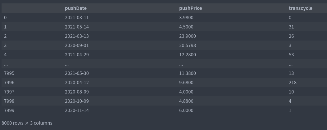
df4 = pd.read_csv('./data/file4.csv')
df5 = pd.read_csv('./data/file5.csv')
(1) Calculate transaction cycle
# Remove unsold samples
df_trans = df4[df4.withdrawDate.notna()]

. . . . Please download the complete code https://mianbaoduo.com/o/bread/YpiXlpZx

train_cols = ['pushDate','pushPrice','transcycle']
df_train = df_trans[train_cols]
test_cols = ['pushDate','pushPrice']
df_test = df5[test_cols]
df_train
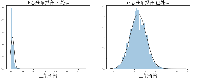
import scipy.stats as st
import seaborn as sns
import matplotlib.pyplot as plt

plt.figure(figsize=(14, 5))
plt.subplot(122)
plt.title('Normal distribution fitting-Processed', fontsize=20)
sns.distplot(np.log1p(df_train['pushPrice']), kde=False, fit=st.norm)
plt.xlabel('Shelf price', fontsize=20)
plt.subplot(121)
plt.title('Normal distribution fitting-Untreated', fontsize=20)
sns.distplot(df_train['pushPrice'], kde=False, fit=st.norm)
plt.xlabel('Shelf price', fontsize=20)
plt.savefig('img/Fitting of normal distribution of on shelf price.png',dpi=300)
(2) Extracting temporal features
# # Processing time (extraction date)
df_train['pushDate'] = pd.to_datetime(df_train['pushDate'])
df_test['pushDate'] = pd.to_datetime(df_test['pushDate'])
df_train['pushDate_year'] = df_train['pushDate'].dt.year
df_train['pushDate_month'] = df_train['pushDate'].dt.month
df_train['pushDate_day'] = df_train['pushDate'].dt.day

df_test['pushDate_year'] = df_test['pushDate'].dt.year
df_test['pushDate_month'] = df_test['pushDate'].dt.month
df_test['pushDate_day'] = df_test['pushDate'].dt.day

del df_train['pushDate']
del df_test['pushDate']
(3) Conversion of data distribution
df_train['pushPrice'] = np.log1p(df_train['pushPrice'])
df_test['pushPrice'] = np.log1p(df_test['pushPrice'])
df_train.columns
Index(['pushPrice', 'update_price', 'barging_times', 'barging_price', 'transcycle', 'pushDate_year', 'pushDate_month', 'pushDate_day'], dtype='object')
(4) Feature crossover
#Define cross feature statistics
def cross_cat_num(df, num_col, cat_col):
    for f1 in tqdm(cat_col):
        g = df.groupby(f1, as_index=False)
        for f2 in tqdm(num_col):
            feat = g[f2].agg({
                '{}_{}_max'.format(f1, f2): 'max', '{}_{}_min'.format(f1, f2): 'min',
                '{}_{}_median'.format(f1, f2): 'median',
                '{}_{}_sum'.format(f1, f2): 'sum',
                '{}_{}_mad'.format(f1, f2): 'mad',
            })
            df = df.merge(feat, on=f1, how='left')
    return(df)
### Cross with numerical features and category features
cross_num = ['pushPrice']

cross_cat = ['pushDate_year', 'pushDate_month','pushDate_day']
data_train = cross_cat_num(df_train, cross_num, cross_cat)  # First order crossover
data_test = cross_cat_num(df_test, cross_num, cross_cat)  # First order crossover
data_train.shape
(8000, 20)
2.3 model training
(1) Model training
from sklearn import metrics
from sklearn.model_selection import KFold
import lightgbm as lgb
import pandas as pd
from sklearn.model_selection import KFold

import numpy as np
from sklearn.preprocessing import StandardScaler

from sklearn.preprocessing import StandardScaler
train = data_train
test = data_test
train_y = train['transcycle']
del train['transcycle']
scaler = StandardScaler()
train_x = scaler.fit_transform(train)
test_x = scaler.fit_transform(test)

from sklearn import metrics

params = {
    'boosting_type': 'gbdt',
    'objective': 'regression_l1',
    'metric': 'mae',
    'num_leaves': 31,
    'learning_rate': 0.05,
    'feature_fraction': 0.9,
    'bagging_fraction': 0.8,
    'bagging_freq': 5,
    'verbose': -1,
}

def MAE_metric(y_true, y_pred):
    return metrics.mean_absolute_error(y_true, y_pred)
folds = 5
kfold = KFold(n_splits=folds, shuffle=True, random_state=5421)
preds_lgb = np.zeros(len(test_x))
for fold, (trn_idx, val_idx) in enumerate(kfold.split(train_x, train_y)):
    import lightgbm as lgb
    print('-------fold {}-------'.format(fold))
    x_tra, y_trn, x_val, y_val = train_x[trn_idx], train_y.iloc[trn_idx], train_x[val_idx], train_y.iloc[val_idx]

    train_set = lgb.Dataset(x_tra, y_trn)
    val_set = lgb.Dataset(x_val, y_val)
    # lgb
    lgbmodel =. . . . Please download the complete code

    val_pred_xgb = lgbmodel.predict(
        x_val, predict_disable_shape_check=True)
    preds_lgb += lgbmodel.predict(test_x,
                                    predict_disable_shape_check=True) / folds
    val_mae = MAE_metric(y_val, val_pred_xgb)
    print('lgb val_mae {}'.format(val_mae))
-------fold 0------- lgb val_mae 15.108706443185115 -
------fold 1------- lgb val_mae 15.755760771009792
-------fold 2------- lgb val_mae 16.597388380375197
-------fold 3------- lgb val_mae 15.483798531878621
-------fold 4------- lgb val_mae 15.278992579304203
(2) Store the prediction results as TXT
import math
file5 = pd.read_csv('./data/file5.csv')
submit_file  = pd.DataFrame(columns=['id'])
submit_file['id'] = file5['carid']
# Round up
submit_file['transcycle'] = [math.ceil(i) for i in list(preds_lgb)]
submit_file['transcycle'].astype(int)

i = 0
with open('./submit/Annex 6: results of store transaction model.txt','a+', encoding='utf-8') as f:
    for line in submit_file.values:
        if i==0:
            i += 1
            continue
        else:
            i += 1
            f.write((str(line[0])+'\t'+str(line[1])+'\n'))
See the top link for complete ideas and code download