19. Scatter plots
19.1. Connected scatter plot
19.2. Bubble chart
19.3. Scatter diagram of different colors
20. Histograms

19. Scatter plots

Use a scatter chart when you want to show the relationship between two variables. Scatter charts are sometimes called correlation charts because they show the relationship between two variables.

import numpy as np
import matplotlib.pyplot as plt

plt.scatter(x=range(77, 770, 10),
            y=np.random.randn(70)*55+range(77, 770, 10),
            s=200, alpha=0.6)
plt.tick_params(labelsize=12)
plt.xlabel('Surface(m2)', size=12)
plt.ylabel('Turnover (K dollars)', size=12)
plt.xlim(left=0)
plt.ylim(bottom=0)

plt.show()

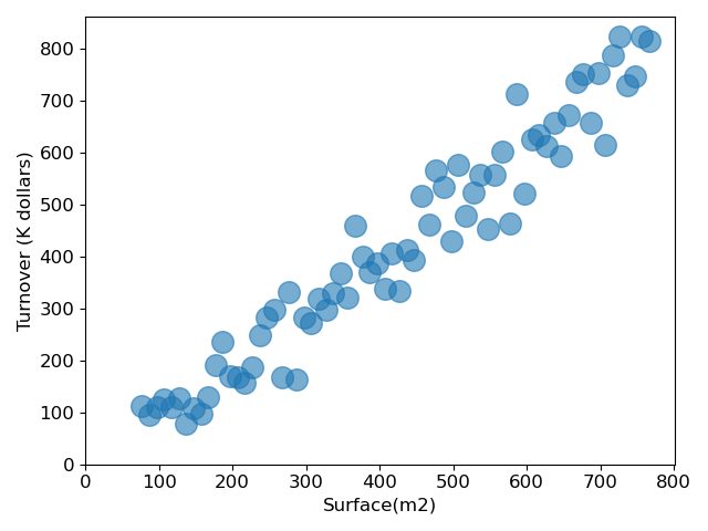
This figure describes the positive correlation between store area and its turnover.

import numpy as np
import matplotlib.pyplot as plt

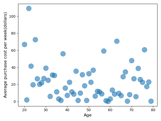
plt.scatter(x=range(20, 80, 1), y=np.abs(np.random.randn(60)*40),
            s=200,
            alpha=0.6)
plt.xlabel('Age', size=12)
plt.ylabel('Average purchase cost per week(dollars)', size=12)

plt.show()

This figure shows that there is no concern between the customer's age and his weekly purchase cost.

19.1. Connected scatter plot

Connected scatter chart is a mixture of scatter chart and line chart. It uses line segments to connect continuous scatter points, for example, to illustrate the trajectory over time.

The connected scatter diagram visualizes two related time series in the scatter diagram and connects these points with lines in the time sequence.

import numpy as np
import matplotlib.pyplot as plt

turnover = [30, 38, 26, 20, 21, 15, 8, 5, 3, 9, 25, 27]
plt.plot(np.arange(12), turnover, marker='o')

plt.show()

Suppose the figure above describes the sales turnover within one year. According to the chart, we can find that sales peak in winter and then decline from spring to summer.

19.2. Bubble chart

A bubble chart is a chart that displays data in three dimensions. The value of an additional variable is represented by the size of the point.

import numpy as np
import matplotlib.pyplot as plt

nbclients = range(10, 494, 7)
plt.scatter(x=range(77, 770, 10),
            y=np.random.randn(70)*55+range(77, 770, 10),
            s=nbclients, alpha=0.6)

plt.show()

19.3. Scatter diagram of different colors

Scatter charts created by matplotlib cannot specify colors based on the values of category variables. Therefore, we must overlap the graphs with different colors.

import numpy as np
import matplotlib.pyplot as plt

plt.scatter(x=range(40, 70, 1),
            y=np.abs(np.random.randn(30)*20),
            s=200,
            #c = 'blue',
            alpha=0.6,
            label='40-69')
plt.scatter(x=range(20, 40, 1),
            y=np.abs(np.random.randn(20)*40),
            s=200,
            #c = 'red',
            alpha=0.6,
            label='20-39')
plt.legend()  # Every time
plt.show()

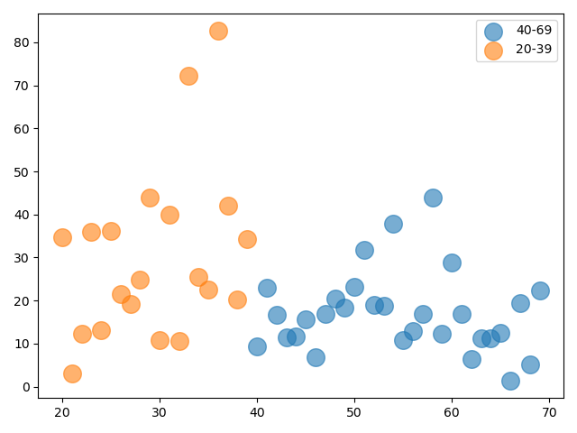
This 2-dot chart clearly shows the difference in weekly purchase costs between young people and middle-aged or elderly people: the average weekly purchase of young people is twice that of middle-aged or elderly people.

20. Histograms

Histogram is a statistical report chart, which is a graphical representation of the frequency distribution of some numerical data. The data distribution is represented by a series of longitudinal stripes or line segments with different heights. Generally, the horizontal axis represents the data type and the vertical axis represents the distribution.

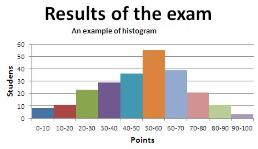
Histogram is a graphical representation of the distribution of numerical data and an estimation of the probability distribution of a continuous variable.

In order to construct the histogram, the first step is to segment the range of values, that is, divide the whole range of values into a series of intervals, and then calculate how many values there are in each interval. These values are usually specified as continuous, non overlapping variable intervals. Intervals must be adjacent and usually of equal size.

If a histogram is constructed, the range of possible x values is first assigned to intervals that are usually equal in size and adjacent.
pyplot.hist function definition document: plot Hist function definition document plot hist( https://matplotlib.org/stable/api/_as_gen/matplotlib.py plot.hist.html )

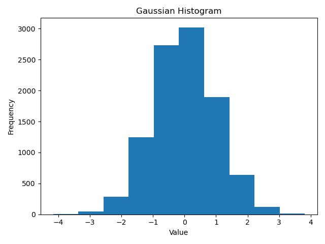
Now let's create a histogram of random numbers:

import matplotlib.pyplot as plt
import numpy as np
gaussian_numbers = np.random.normal(size=10000)
print(gaussian_numbers)
'''
Output result:
[-2.88618646 -0.15302214 -0.35230715 ... -0.42074156  0.41650123 0.56230326]
'''

plt.hist(gaussian_numbers)
plt.title("Gaussian Histogram")
plt.xlabel("Value")
plt.ylabel("Frequency")
plt.show()

Return value:
n The values of the histogram bins.
bins
The edges of the bins. Length nbins + 1 (nbins left edges and right edge of last bin).
patches
Silent list of individual patches used to create the histogram or list of such list if multiple input datasets.

import matplotlib.pyplot as plt
import numpy as np
gaussian_numbers = np.random.normal(size=10000)
print(gaussian_numbers)
'''
Output result:
[-2.88618646 -0.15302214 -0.35230715 ... -0.42074156  0.41650123 0.56230326]
'''


n, bins, patches = plt.hist(gaussian_numbers)
print("n: ", n, sum(n))
print("bins: ", bins)
for i in range(len(bins)-1):
    print(bins[i+1] -bins[i])
print("patches: ", patches)
print(patches[1])
"""
Output result:
n:  [  25.  182.  940. 2230. 2951. 2268. 1066.  300.   34.    4.] 10000.0
bins:  [-3.44422377 -2.68683456 -1.92944534 -1.17205613 -0.41466692  0.3427223
  1.10011151  1.85750072  2.61488994  3.37227915  4.12966836]
0.7573892130572868
0.757389213057287
0.757389213057287
0.7573892130572868
0.7573892130572868
0.7573892130572872
0.7573892130572863
0.7573892130572872
0.7573892130572872
0.7573892130572859
patches:  <BarContainer object of 10 artists>
Rectangle(xy=(-2.68683, 0), width=0.757389, height=182, angle=0)
"""

plt.title("Gaussian Histogram")
plt.xlabel("Value")
plt.ylabel("Frequency")
plt.show()

Parameter Description:
 data: required parameter, drawing data
 bins: the number of long bars in the histogram. Optional. The default value is 10
 normalized: whether to normalize the obtained histogram vector. Optional. The default value is 0, which represents non normalization and display frequency. Normalized = 1, indicating normalization and displaying frequency.
 facecolor: color of long strip
 edgecolor: the color of the long bar border
• alpha: transparency

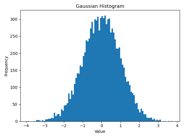
Let's increase the number of bin. If there are 10000 random values, set the keyword parameter bins to 100:

plt.hist(gaussian_numbers, bins=100)
plt.show()

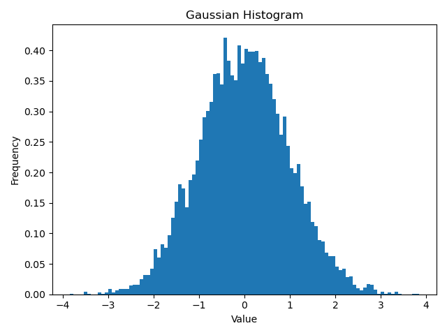
Another important keyword parameter of hist is density. Density is optional and the default value is False. If it is set to True, the first element of the returned tuple will be normalized to form the count value of probability density, that is, the sum of the area (or integral) under the histogram is 1.

plt.hist(gaussian_numbers, bins=100, density=True)
plt.show()

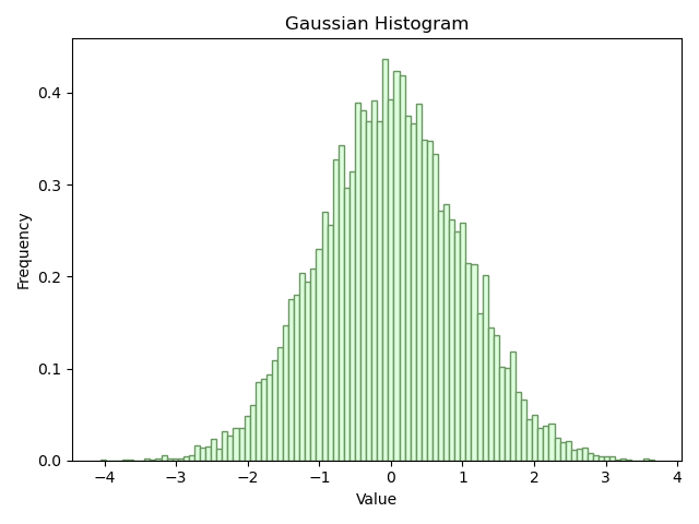
hist to set edgecolor and color.

plt.hist(gaussian_numbers, 
         bins=100, 
         density=True, 
         edgecolor="#6A9662",
         color="#DDFFDD")
plt.show()

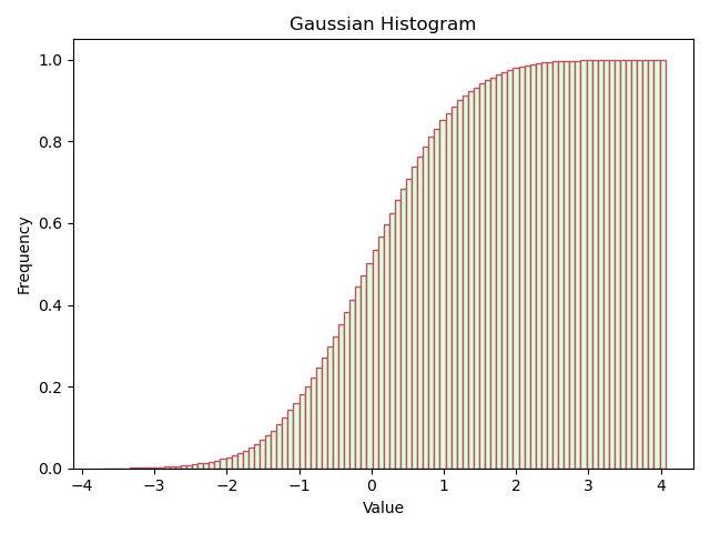
By setting the parameter cumulative, we can also draw it as a cumulative distribution function.

n, bins, patches = plt.hist(gaussian_numbers,
                            bins=100,
                            density=True,
                            edgecolor="#BB5566",
                            color="#DDFFDD",
                            cumulative=True)
plt.show()