1. Introduction
A* (A-Star) algorithm is a solution in static road network Shortest path One of the most effective methods is a commonly used heuristic algorithm
Heuristic algorithm: calculate the key value through heuristic function to guide the search direction of the algorithm
2. Algorithm description
Ray Wenderlich - Introduction to A* Pathfinding
This article very well introduces the logic of A * algorithm and its key points, and English is easy to understand, so this article will not translate this blog in detail
In short, a * algorithm starts from the starting point, selects the point with the minimum key value by calculating the key value of adjacent reachable points and comparing it with other optional points, and then continues to calculate the key value of adjacent points of this point until it reaches the end point Imagine that like a stone falling into the water, the ripples of the water diffuse outside, and the circles of ripples can be regarded as points with the same key value A * algorithm does not need to traverse all points. On the contrary, if the heuristic function, that is, the closer the distance estimation of the current point is to the actual value, a * algorithm will move to the end along the shortest path to avoid traversing points with high key value
Therefore, the key of the algorithm is to use the OPEN and CLOSE lists to record the access points and how to calculate the key values
2.1 OPEN and CLOSE lists
OPEN list: A list of all alternative points under consideration. This table is not A list of all points, but the points that can be reached by A * algorithm when calculating adjacent points
CLOSE list: a list of all accessed points
When the point with the minimum key value is selected from all adjacent reachable points, this point will be placed in the CLOSE list, and the other points will be placed in the OPEN list
2.2 key value calculation F = G+H
G Value: represents the cost from the starting point to the current point
H value: represents the cost from the current point to the end point. Since starting from the current point, we do not know how to reach the end point, so this value is the value estimated by the heuristic function
It should be noted that if the key value F of the calculated adjacent point (the adjacent point is already in OPEN) is less than the stored key value, it means that there is a better path to the adjacent point, the key value and G value of the adjacent point need to be updated
2.3 H (heuristic)
Baidu Encyclopedia's choice of h(n)
The estimated distance from the state n to the target state is expressed in h(n), and h*(n) represents the actual distance. Then the selection of h(n) is roughly as follows:
-
If h (n) < h * (n), in this case, the number of search points is large, the search range is large, and the efficiency is low. But the optimal solution can be obtained.
-
If h(n)=h*(n), the search efficiency is the highest.
-
If h (n) > h * (n), the number of search points is small, the search range is small and the efficiency is high, but the optimal solution can not be guaranteed.
The usual heuristic functions can include Manhattan distance, diagonal distance, Euclidean distance, etc., or establish heuristic equations according to the actual situation
Detailed explanation of the best and most complete A * algorithm (translation) This blog post has a more in - depth discussion on the selection of heuristic functions
Manhattan distance
h(n) = D*(abs(a.x - b.x ) + abs(a.y - b.y ))
Diagonal distance
h(n) = D*max(abs(a.x - b.x), abs(a.y - b.y))
Euclidean distance
h(n) = D*sqrt((a.x - b.x)^2 + (a.y - b.y)^2)
Note that the selection of heuristic function is also related to how to reach adjacent points. For example, if you can only move up, down, left and right to reach adjacent points, the selection of diagonal distance is inappropriate
2.4 algorithm loop exit conditions:
1) Find the shortest path from the beginning to the end
2) The path cannot be found by traversing all points (the OPEN list is finally empty)
3. Examples
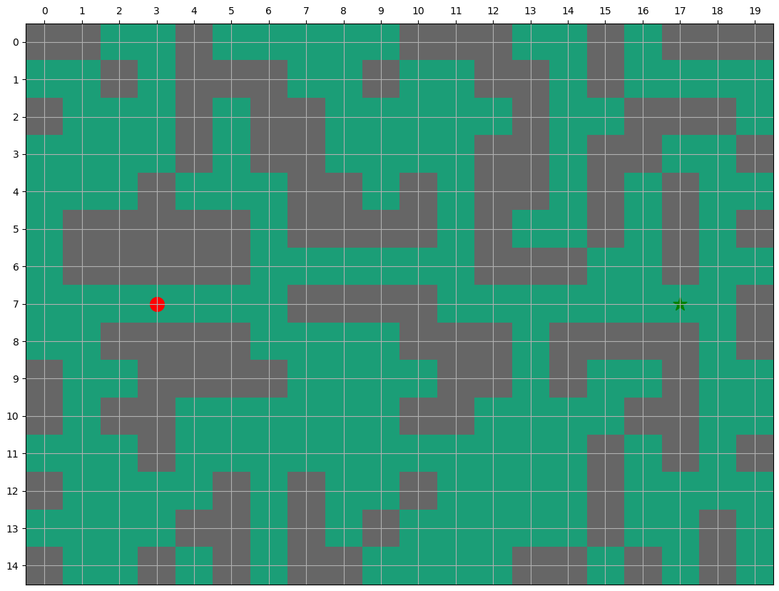
Find the shortest path from (7, 3) to (7, 13) in the figure below

4. Python code implementation
import numpy as np
import heapq
import matplotlib.pyplot as plt
import time


# def heuristic(a, b):
#     return np.sqrt((b[0] - a[0]) ** 2 + (b[1] - a[1]) ** 2)

def heuristic(a, b):
    return abs(a[0]-b[0]) + abs(a[1]-b[1])


def astar(array, start, goal):
    close_set = set()
    parent_from_dict = {}
    gscore = {start: 0}
    fscore = {start: heuristic(start, goal)}
    open_list = []
    heapq.heappush(open_list, (fscore[start], start))
    while open_list:
        current = heapq.heappop(open_list)[1]  # return the smallest value
        if current == goal:
            route_loc = []
            while current in parent_from_dict:
                route_loc.append(current)
                current = parent_from_dict[current]
            # append start point to route and reorder route backward to get correct node sequence
            route_loc = route_loc + [start]
            route_loc = route_loc[::-1]
            return route_loc, close_set, open_list

        close_set.add(current)

        for i, j in neighbor_direction:
            neighbor = current[0] + i, current[1] + j
            tentative_g_score = gscore[current] + heuristic(current, neighbor)
            if 0 <= neighbor[0] < array.shape[0]:
                if 0 <= neighbor[1] < array.shape[1]:
                    if array[neighbor[0]][neighbor[1]] == 1:
                        # print('neighbor %s hit wall' % str(neighbor))
                        continue
                else:
                    # array bound y walls
                    # print('neighbor %s hit y walls' % str(neighbor))
                    continue
            else:
                # array bound x walls
                # print('neighbor %s hit x walls' % str(neighbor))
                continue

            if neighbor in close_set and tentative_g_score >= gscore.get(neighbor, 0):
                continue

            if tentative_g_score < gscore.get(neighbor, 0) or neighbor not in [i[1] for i in open_list]:
                parent_from_dict[neighbor] = current
                gscore[neighbor] = tentative_g_score
                fscore[neighbor] = tentative_g_score + heuristic(neighbor, goal)
                heapq.heappush(open_list, (fscore[neighbor], neighbor))
    return None, close_set, open_list


def plot(layout, path=None, close_set=None, open_set=None):
    fig, ax = plt.subplots(figsize=(20, 20))
    ax.imshow(layout, cmap=plt.cm.Dark2)

    ax.scatter(start[1], start[0], marker="o", color="red", s=200)
    ax.scatter(goal[1], goal[0], marker="*", color="green", s=200)

    if path:
        # extract x and y coordinates from route list
        x_coords = []
        y_coords = []
        for k in (range(0, len(path))):
            x = path[k][0]
            y = path[k][1]
            x_coords.append(x)
            y_coords.append(y)

        ax.plot(y_coords, x_coords, color="black")

    if close_set:
        for c in close_set:
            ax.scatter(c[1], c[0], marker='o', color='green')

    if open_set:
        for p in open_set:
            loc = p[1]
            ax.scatter(loc[1], loc[0], marker='x', color='blue')

    ax.xaxis.set_ticks(np.arange(0, layout.shape[1], 1))
    ax.yaxis.set_ticks(np.arange(0, layout.shape[0], 1))
    ax.xaxis.tick_top()
    plt.grid()
    plt.show()


if __name__ == '__main__':
    # neighbor_direction = [(0, 1), (0, -1), (1, 0), (-1, 0), (1, 1), (1, -1), (-1, 1), (-1, -1)]
    neighbor_direction = [(0, 1), (0, -1), (1, 0), (-1, 0)]

    S = np.array([
        [1, 1, 0, 0, 1, 0, 0, 0, 0, 0, 1, 1, 1, 0, 0, 1, 0, 1, 1, 1],
        [0, 0, 1, 0, 1, 1, 1, 0, 0, 1, 0, 0, 1, 1, 0, 1, 0, 0, 0, 0],
        [1, 0, 0, 0, 1, 0, 1, 1, 0, 0, 0, 0, 0, 1, 0, 0, 1, 1, 1, 0],
        [0, 0, 0, 0, 1, 0, 1, 1, 0, 0, 0, 0, 1, 1, 0, 1, 1, 0, 0, 1],
        [0, 0, 0, 1, 0, 0, 0, 1, 1, 0, 1, 0, 1, 1, 0, 1, 0, 1, 0, 0],
        [0, 1, 1, 1, 1, 1, 0, 1, 1, 1, 1, 0, 1, 0, 0, 1, 0, 1, 0, 1],
        [0, 1, 1, 1, 1, 1, 0, 0, 0, 0, 0, 0, 1, 1, 1, 0, 0, 1, 0, 0],
        [0, 0, 0, 0, 0, 0, 0, 1, 1, 1, 1, 0, 0, 0, 0, 0, 0, 0, 0, 1],
        [0, 0, 1, 1, 1, 1, 0, 0, 0, 0, 1, 1, 1, 0, 1, 1, 1, 1, 0, 1],
        [1, 0, 0, 1, 1, 1, 1, 0, 0, 0, 0, 1, 1, 0, 1, 0, 0, 1, 0, 0],
        [1, 0, 1, 1, 0, 0, 0, 0, 0, 0, 1, 1, 0, 0, 0, 0, 1, 1, 0, 0],
        [0, 0, 0, 1, 0, 0, 0, 0, 0, 0, 0, 0, 0, 0, 0, 1, 0, 1, 0, 1],
        [1, 0, 0, 0, 0, 1, 0, 1, 0, 0, 1, 0, 0, 0, 0, 1, 0, 0, 0, 0],
        [0, 0, 0, 0, 1, 1, 0, 1, 0, 1, 0, 0, 0, 0, 0, 1, 0, 0, 1, 0],
        [1, 0, 0, 1, 0, 1, 0, 1, 1, 0, 0, 0, 0, 1, 1, 0, 1, 0, 1, 0],
    ])

    start = (7, 3)
    goal = (7, 17)

    # S[(7, 12)] = 1
    # S[(7, 15)] = 1

    t_start = time.perf_counter()
    route, c_set, open_l = astar(S, start, goal)
    t_end = time.perf_counter()
    print(f"astar finished in {t_end - t_start:0.4f} seconds")
    if route:
        print(route)
        plot(S, route, c_set, open_l)
    else:
        plot(S, None, c_set, open_l)
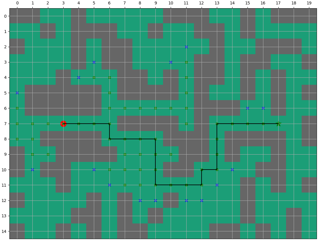
It can be seen from the figure above that the algorithm only calculates a very few points in the figure, that is, it finds the end point (green "o" represents the point in CLOSE and blue "x" represents the point in OPEN)

The figure above shows the shortest path when (7,12) has obstacles. At this time, it can be seen that the points calculated by A * algorithm greatly exceed those without obstacles, but the algorithm is always effective and does not traverse all points

The above figure shows that when the A * algorithm cannot find the path, it can be seen that the algorithm traverses all possible points (green "o" represents the points in CLOSE)
4. Algorithm summary
A * algorithm can quickly find the path from the starting point to the end point, and can control and decide whether to get the shortest path or a suboptimal path through different heuristic functions. When the calculation time is very long