Serial article:
Last Vernacular machine learning concepts

1, Machine learning category

Machine learning can be divided into supervised learning, unsupervised learning, semi supervised learning and reinforcement learning according to the difference of learning data experience, that is, the difference of label information of training data.

1.1 supervised learning

Supervised learning is the most widely used and mature in machine learning. It learns how to associate x to the correct y from the labeled data samples (x, y). This process is like the model learning with reference to the answer (label y) under the known conditions (feature x) of a given question. With the help of label Y's supervision and correction, the model continuously adjusts its parameters through the algorithm to achieve the learning goal.

The commonly used models for supervised learning include linear regression, naive Bayes, K-nearest neighbor, logical regression, support vector machine, neural network, decision tree, integrated learning (such as LightGBM), etc. according to the application scenario, if the value of Y predicted by the model is limited or infinite, it can be further divided into classification or regression models.

Classification model

The classification model is to deal with the classification task with limited value of prediction results. The following example uses a logistic regression classification model to predict whether it will rain according to temperature, humidity, wind speed, etc.

• Introduction to logistic regression

Although the name of logistic regression has "regression", in fact, it is a generalized linear classification model. Because the model is simple and efficient, it is widely used in practice.

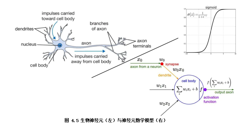
The structure of the logistic regression model can be regarded as a two-layer neural network (as shown in Fig. 4.5). The model input x, the input nonlinearity is converted to the value output of 0 ~ 1 through the neuron activation function f (F is the sigmoid function), and the final learned model decision function is Y=sigmoid(wx + b)

. The model parameter w is the weight (w1,w2,w3...) corresponding to each feature (x1, x2, x3...), the model parameter b represents the bias term, and Y is the prediction result (0 ~ 1 range).

The learning goal of the model is to minimize the cross entropy loss function. The optimization algorithm of the model often uses the gradient descent algorithm to iteratively solve the minimum of the loss function to obtain better model parameters.

• Code example
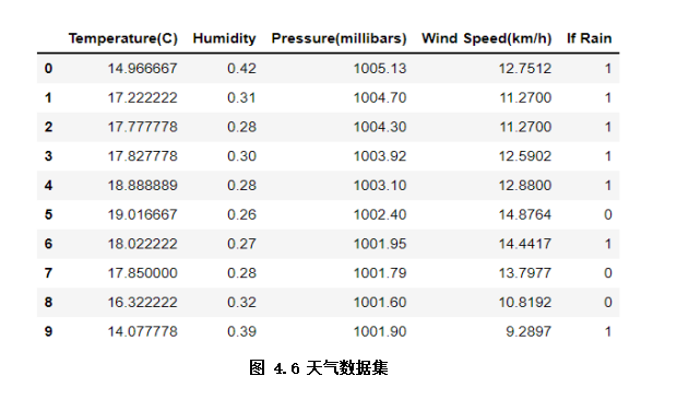
  The weather data set used in the example is simple weather record data, including outdoor temperature and humidity, wind speed, rain, etc. in the classification task, we take rain as the label and others as the characteristics (as shown in Figure 4.6)
  

import pandas as pd    # Import pandas Library
weather_df = pd.read_csv('./data/weather.csv')   # Load weather dataset
weather_df.head(10)   # Display the first 10 rows of data

from sklearn.linear_model import LogisticRegression  # Import logistic regression model
x = weather_df.drop('If Rain', axis=1)  # Characteristic x
y = weather_df['If Rain']  # Label y
lr = LogisticRegression()
lr.fit(x, y)  # model training
print("Prediction results of the first 10 samples:", lr.predict(x[0:10]) ) # The model predicts the first 10 samples and outputs the results

The prediction results of the first 10 samples output by the trained model are: [1 1 1 1 1 0 1 1 1 1 1 1 1 1 1 1 1 1 1 1 1 1 1 0 1 0 1 1 1 1 1 1 0 1 1 1 1 1 1 1 0 1 1 1 1 1 1 1 1 1 1 1 0 1 1 1 1 1 1 1 1 1 1 1 1 1 1 1 1 1 1 1 1 1 1 1 1 1 1 1 1 1 1 1 1 1 1 1 1. In the following chapters, we will specifically introduce how to evaluate the prediction effect of the model and further optimize the model effect.

regression model
Regression model is a regression task to deal with the infinite value of prediction results. The following code example uses the linear regression model to predict the outdoor humidity according to the temperature, wind, rain and other conditions with the outdoor humidity as the label.

• Introduction to linear regression
  The premise of linear regression model is that y and X are linear, input x, and the decision function of the model is Y=wx+b. The learning goal of the model is to minimize the mean square error loss function. The optimization algorithm of the model usually uses the least square method to solve the optimal model parameters.
• Code example

from sklearn.linear_model import LinearRegression  #Import linear regression model
x = weather_df.drop('Humidity', axis=1)  # Characteristic x
y = weather_df['Humidity']  # Label y
linear = LinearRegression()

linear.fit(x, y)  # model training
print("Prediction results of the first 10 samples:", linear.predict(x[0:10]) ) # The model predicts the first 10 samples and outputs the results
# Prediction results of the first 10 samples: [0.42053525 0.32811401 0.31466161 0.3238797 0.29984453 0.29880059

1.2 unsupervised learning

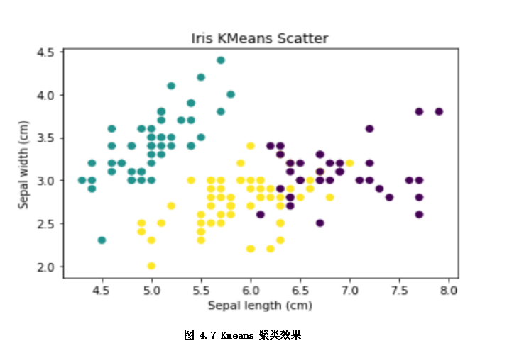
Unsupervised learning is also widely used in machine learning, It is to learn the internal laws of data from unmarked data (x). This process is like a model in which no one provides reference answers (y) , summarize and summarize the knowledge points completely through thinking about the knowledge points of the topic. According to the application scenario, unsupervised learning can be divided into clustering, feature reduction and association analysis. The following example divides iris iris samples of different varieties through Kmeans clustering.

• Introduction to Kmeans clustering
  Kmeans clustering is a common method of unsupervised learning. Its principle is to initialize k cluster centers and update each cluster sample through iterative algorithm to achieve the goal of minimizing the distance between the sample and the cluster center to which it belongs. The algorithm steps are as follows:
  1. Initialization: randomly select k samples as the initial cluster center (the value of K can be determined by prior knowledge and verification method);
  2. Calculate the distance from each sample in the data set to the center of k cluster classes, and assign it to the class corresponding to the center of the cluster class with the smallest distance;
  3. Recalculate the center position of each cluster class;
  4. Repeat the above steps 2 and 3 until a certain termination condition is reached (such as the number of iterations, the center position of the cluster class remains unchanged, etc.)

• Code example

from sklearn.datasets import load_iris  # data set
from sklearn.cluster import KMeans   #  Kmeans model
import matplotlib.pyplot as plt  # plt drawing
lris_df = datasets.load_iris()  # The iris iris iris data set is loaded. There are 150 samples in the data set, which are divided into three types of iris varieties
x = lris_df.data
k = 3  # k clusters are clustered. There are three types of varieties in the known data set, which is set as 3
model = KMeans(n_clusters=k)  
model.fit(x)  # Training model
print("Clustering results of the first 10 samples:",model.predict(x[0:10]) ) # The model predicts the first 10 samples and outputs the clustering results: [1 1 1 1 1 1 1 1 1 1 1 1 1 1 1 1 1 1 1 1 1 1 1 1 1 1 1 1 1 1 1 1 1 1 
# The clustering effect of samples is shown by scatter diagram
x_axis = lris_df.data[:,0] # The sepal length (cm) of iris flower was used as the x-axis
y_axis = lris_df.data[:,1] # The sepal width (cm) of iris flower was used as the y-axis
plt.scatter(x_axis, y_axis, c=model.predict(x)) # The sub label color shows the clustering effect
plt.xlabel('Sepal length (cm)')#Set x-axis annotation
plt.ylabel('Sepal width (cm)')#Set y-axis annotation
plt.title('Iris KMeans Scatter')
plt.show()   # As shown in Figure 4.7, clustering effect

1.3 semi supervised learning

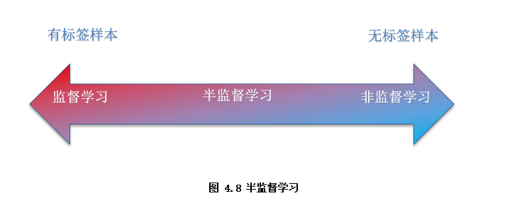
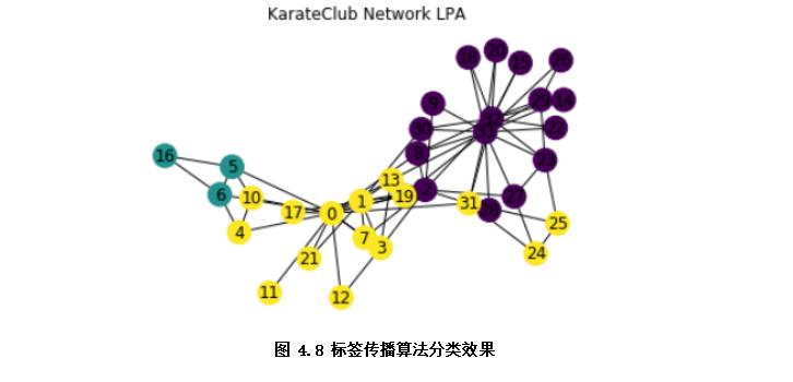
Semi supervised learning is between traditional supervised learning and unsupervised learning (as shown in Figure 4.8), the idea is to introduce unlabeled samples into model training under certain assumptions when the number of labeled samples is small, so as to fully capture the overall potential distribution of data and improve the problems such as blindness of traditional unsupervised learning process and poor learning effect caused by insufficient training samples of supervised learning. According to application scenarios, semi supervised learning can be divided into For clustering, classification and regression methods. The following example classifies club members through a graph based semi supervised algorithm, label propagation algorithm.

-Introduction to label propagation algorithm

Label propagation algorithm (LPA) is a graph based semi supervised learning classification algorithm. The basic idea is to predict the unlabeled node labels from the labeled node label information in the graph network composed of all samples.

1. Firstly, the complete graph model is established by using the relationship between samples (which can be the objective relationship of samples, or the relationship between samples is calculated by similarity function).

2. Then add the labeled label information (or none) to the graph. The unlabeled node is initialized with a random unique label.

3. Set the label of a node as the label with the highest frequency among the adjacent nodes of the node, and repeat the iteration until the label remains unchanged, that is, the algorithm converges.

-Code example
The sample dataset karate club is a widely used social network, in which nodes represent members of karate club and edges represent the relationship between members.

import networkx as nx # Import networkx diagram Library
import matplotlib.pyplot as plt
from networkx.algorithms import community  # Graph community algorithm
G=nx.karate_club_graph()   # Load American Karate Club map data
#Note: this example does not use marked information. Strictly speaking, it is an unsupervised application case of semi supervised algorithm
lpa = community.label_propagation_communities(G)  # Run label propagation algorithm
community_index = {n: i for i, com in enumerate(lpa) for n in com} # Node corresponding to each label
node_color = [community_index[n] for n in G]  # Use label as node color
pos = nx.spring_layout(G)  # The layout of nodes is spring type
nx.draw_networkx_labels(G, pos) # Node serial number
nx.draw(G, pos, node_color=node_color) # Sub label color display network
plt.title(' Karate_club network LPA')
plt.show() #Show the classification effect. Different colors are different categories

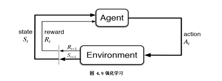
1.4 reinforcement learning

Reinforcement learning can be regarded as supervised learning with delayed label information to some extent (as shown in Figure 4.9), it refers to the learning process in which the Agent takes a behavior action in the Environment, which is transformed into a reward and a state representation state, and then fed back to the Agent. In this book, reinforcement learning is only briefly introduced, and can be expanded if interested.

The article starts with algorithm, and the official account reads the original text. GitHub project source code