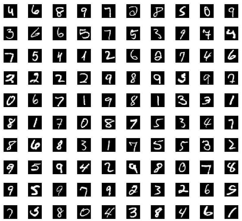
The handwriting database is used. The database has been integrated into the toolbox. Just use it directly. Show a part of the database. The goal is to train the database to achieve the purpose of recognition:
Then, the database data is normalized and preprocessed. nnsetup establishes a network, in which many parameters will be initialized, and opts numepochs = 1; The personal feeling of this parameter is to repeat the test times for all data, and setting 1 is to experiment once. opts.batchsize = 100; This parameter is to send a large number of samples every 100 at random as a wave into the experiment. Then there's the training test.
nnsetup:
function nn = nnsetup(architecture)
%NNSETUP Create forward neural network
% nn = nnsetup(architecture) Returns a neural network structure, architecture Is a structural parameter
% architecture It's a n x 1 Vector representing the number of neurons in each layer
%such as architecture=[784 100 10],Indicates that the input layer is 784 dimensional input, 100 hidden layers and 10 output layers
%Why is the input 784: because each handwriting size is 28*28 That is, the 784 dimension
%Why the hidden layer is 100: it can be set freely, can be modified freely, and needs to be designed
%Why is the output 10: the handwriting has 0-9 These 10 results, so it is 10

    nn.size   = architecture;
    nn.n      = numel(nn.size);

    nn.activation_function              = 'tanh_opt';   % Hidden layer activation function: 'sigm' (sigmoid) or 'tanh_opt' (default tanh).
    nn.learningRate                     = 2;            %  Learning rate: typically needs to be lower when using 'sigm' activation function and non-normalized inputs.
    nn.momentum                         = 0.5;          %  Momentum Weight momentum factor
    nn.scaling_learningRate             = 1;            %  Learning rate change factor (each epoch)
    nn.weightPenaltyL2                  = 0;            %  L2 regularization Regularization
    nn.nonSparsityPenalty               = 0;            %  Non sparse penalty
    nn.sparsityTarget                   = 0.05;         %  Sparse target value
    nn.inputZeroMaskedFraction          = 0;            %  Denoising effect of automatic coding
    nn.dropoutFraction                  = 0;            %  Dropout level (http://www.cs.toronto.edu/~hinton/absps/dropout.pdf)
    nn.testing                          = 0;            %  Internal variable. nntest sets this to one.
    nn.output                           = 'sigm';       %  Output activation output unit 'sigm' (=logistic), 'softmax' and 'linear'

    for i = 2 : nn.n
        % weights and weight momentum
        nn.W{i - 1} = (rand(nn.size(i), nn.size(i - 1)+1) - 0.5) * 2 * 4 * sqrt(6 / (nn.size(i) + nn.size(i - 1)));
        nn.vW{i - 1} = zeros(size(nn.W{i - 1}));

        % average activations (for use with sparsity)
        nn.p{i}     = zeros(1, nn.size(i));
    end
end
This function is very simple to understand. It initializes the network. What does the network need to initialize, A lot of initialization is suitable for all networks (cnn,dbn, etc.). Now you only need to know the structure of the network and the parameters related to sparse coding representation: nn.nonSparsityPenalty, nn.sparsityTarget, which is why the sparse representation and the specific methods do not need to be controlled. In actual use, there are only a few parameter settings. Let's leave the rest to the program. Then Yes, just notice the activation function NN activation_ function. , Then the network weights are initialized randomly.
Let's talk about the whole function: [nn, L] = nntrain(nn, train_x, train_y, opts);
It can be seen that what nntrain needs is the designed network nn and training data train_x. Training corresponding target value train_y. And the additional parameter opts. Additional parameters include: number of repeated training, opts Numepochs, the size of each block of training data, opts Batch size, etc. The function comes out of the trained network nn, which is very important. The trained nn is the structure, which includes all the information you need, such as the weight coefficient of each layer of network, training error, etc. you can find it, and this trained nn is also used in nntest. See the introduction of the blog above for the specific implementation details of nntrain.
nntrain
setup is about this process. Next, we'll get to train. Open \ NN \ nntrain m
We skip the code that verifies that the incoming data is correct and go straight to the key parts
For the denoising part, please refer to the paper: extracting and composing robot features with denoising autoencoders
m = size(train_x, 1);
//m is the number of training samples
//Note that we set opt when calling. Batch size is the size of batch gradient
batchsize = opts.batchsize; numepochs = opts.numepochs;
numbatches = m / batchsize;  //Calculate the number of batches. Divide the total number of training samples by the size of a batch to get the total number of batches
assert(rem(numbatches, 1) == 0, 'numbatches must be a integer');//That is, the total data is grouped in the previous step, and the number of groups should be an integer
L = zeros(numepochs*numbatches,1);
n = 1;
//numepochs is the number of cycles
for i = 1 : numepochs
    tic;  // tic is used to save the current time, and then toc is used to record the program completion time.
    kk = randperm(m);
    //The random perm (m) function is to randomly disrupt a number sequence and generate an array of 1 to M. For example, randperm(5), ans = 2 3 4 1 5

    for l = 1 : numbatches
        batch_x = train_x(kk((l - 1) * batchsize + 1 : l * batchsize), :);
        //Add noise to input (for use in denoising autoencoder)
        //Add noise, which is the part that denoising autoencoder needs to use
        //For this part, please refer to the paper "extracting and composing robot features with denoising autoencoders"
        //The specific method is to adjust some data in the training sample to 0. inputZeroMaskedFraction represents the adjusted proportion
        if(nn.inputZeroMaskedFraction ~= 0)
            batch_x = batch_x*
(rand(size(batch_x))>nn.inputZeroMaskedFraction);
        end
        batch_y = train_y(kk((l - 1) * batchsize + 1 : l * batchsize), :);
        //These three functions
        //nnff is forward propagation, nnbp is backward propagation, and nnapplygrads is gradient descent
        //We analyze the code of these functions below
        nn = nnff(nn, batch_x, batch_y);
        nn = nnbp(nn);
        nn = nnapplygrads(nn);
        L(n) = nn.L;
        n = n + 1;
    end

    t = toc;
    if ishandle(fhandle)
        if opts.validation == 1
            loss = nneval(nn, loss, train_x, train_y, val_x, val_y);
        else
            loss = nneval(nn, loss, train_x, train_y);
        end
        nnupdatefigures(nn, fhandle, loss, opts, i);
    end

    disp(['epoch ' num2str(i) '/' num2str(opts.numepochs) '. Took ' num2str(t) ' seconds' '. Mean squared error on training set is ' num2str(mean(L((n-numbatches):(n-1))))]);
    nn.learningRate = nn.learningRate * nn.scaling_learningRate;
end
The three functions nnff,nnbp and nnapplygrads are analyzed below
nnff
nnff is a feed forward pass. In fact, it is very simple, that is, the whole network can run forward once
Of course, there are calculations of dropout and sparsity
For details, see the paper "Improving Neural Networks with Dropout" and Autoencoders and Sparsity
function nn = nnff(nn, x, y)
//NNFF performs a feedforward pass
// nn = nnff(nn, x, y) returns an neural network structure with updated
// layer activations, error and loss (nn.a, nn.e and nn.L)

    n = nn.n;
    m = size(x, 1);

    x = [ones(m,1) x];
    nn.a{1} = x;

    //feedforward pass
    for i = 2 : n-1
        //Forward propagation calculation is performed according to different activation functions selected
        //You can look back at the first parameter activation in nnsetup_ function
        //sigm is the sigmoid function, tanh_opt is the function of tanh. The toolbox seems to have changed a little
        //tanh_opt is 1.7159*tanh(2/3.*A)
        switch nn.activation_function
            case 'sigm'
                // Calculate the unit's outputs (including the bias term)
                nn.a{i} = sigm(nn.a{i - 1} * nn.W{i - 1}');
            case 'tanh_opt'
                nn.a{i} = tanh_opt(nn.a{i - 1} * nn.W{i - 1}');
        end

        //dropout fraction is a parameter that can be set in nnsetup
        if(nn.dropoutFraction > 0)
            if(nn.testing)
                nn.a{i} = nn.a{i}.*(1 - nn.dropoutFraction);
            else
                nn.dropOutMask{i} = (rand(size(nn.a{i}))>nn.dropoutFraction);
                nn.a{i} = nn.a{i}.*nn.dropOutMask{i};
            end
        end
        //Calculate sparsity. nonSparsityPenalty is the penalty coefficient for parameters that fail to reach sparsitytarget
        //calculate running exponential activations for use with sparsity
        if(nn.nonSparsityPenalty>0)
            nn.p{i} = 0.99 * nn.p{i} + 0.01 * mean(nn.a{i}, 1);
        end

        //Add the bias term
        nn.a{i} = [ones(m,1) nn.a{i}];
    end
    switch nn.output
        case 'sigm'
            nn.a{n} = sigm(nn.a{n - 1} * nn.W{n - 1}');
        case 'linear'
            nn.a{n} = nn.a{n - 1} * nn.W{n - 1}';
        case 'softmax'
            nn.a{n} = nn.a{n - 1} * nn.W{n - 1}';//N here is the specific number in the loop n-1, representing the last output layer (not participating in the loop)
            nn.a{n} = exp(bsxfun(@minus, nn.a{n}, max(nn.a{n},[],2)));
//max this expression means to compare and take the maximum value of each row, and the result is a column vector.
            nn.a{n} = bsxfun(@rdivide, nn.a{n}, sum(nn.a{n}, 2));
     // bsxfun stands for efficient operation, which refers to the binary operation of calculating elements one by one between two arrays, @ rdivide here refers to left division@ minus is subtraction

    end
    //error and loss

    //Calculation error
    nn.e = y - nn.a{n};
    //Calculate loss function
    switch nn.output
        case {'sigm', 'linear'}
            nn.L = 1/2 * sum(sum(nn.e .^ 2)) / m;
        case 'softmax'
            nn.L = -sum(sum(y .* log(nn.a{n}))) / m;
    end
end
nnbp
Code: \ NN \ nnbp m
nnbp is the process of back propagation, which is more regular than that in ufldl Neural Network Basically the same
It is also worth noting the dropout and sparsity parts
if(nn.nonSparsityPenalty>0)
    pi = repmat(nn.p{i}, size(nn.a{i}, 1), 1);
    sparsityError = [zeros(size(nn.a{i},1),1) nn.nonSparsityPenalty * (-nn.sparsityTarget ./ pi + (1 - nn.sparsityTarget) ./ (1 - pi))];
end

// Backpropagate first derivatives
if i+1==n % in this case in d{n} there is not the bias term to be removed
    d{i} = (d{i + 1} * nn.W{i} + sparsityError) .* d_act; // Bishop (5.56)
else // in this case in d{i} the bias term has to be removed
    d{i} = (d{i + 1}(:,2:end) * nn.W{i} + sparsityError) .* d_act;
end

if(nn.dropoutFraction>0)
    d{i} = d{i} .* [ones(size(d{i},1),1) nn.dropOutMask{i}];
end
This is only the content of the implementation. d{i} in the code is the delta value of this layer, which is described in ufldl
dW{i} is basically the gradient of calculation, but some things need to be added and modified later
See the paper "Improving Neural Networks with Dropout" and Autoencoders and Sparsity Content of
nnapplygrads
Code file: \ NN \ nnapplygrads m
for i = 1 : (nn.n - 1)
    if(nn.weightPenaltyL2>0)
        dW = nn.dW{i} + nn.weightPenaltyL2 * nn.W{i};
    else
        dW = nn.dW{i};
    end

    dW = nn.learningRate * dW;

    if(nn.momentum>0)
        nn.vW{i} = nn.momentum*nn.vW{i} + dW;
        dW = nn.vW{i};
    end

    nn.W{i} = nn.W{i} - dW;
end
This content is simple, NN Weightpenaltyl2 is part of weight decay and a parameter that can be set during nnsetup
If yes, add weight Penalty to prevent over fitting, then adjust it according to the size of momentum, and finally change NN W {I} is enough
nntest
Ok, let's take another look at nntest, as follows:
function [ri, right] = nntest(nn, x, y)
    labels = nnpredict(nn, x);
    [~, expected] = max(y,[],2);
    right = find(labels == expected);
    ri = numel(right) / size(x, 1);
end
Call nnpredict. The function needs test data X and label y. if there is y, the accuracy can be calculated. If there is no y, you can directly call labels = nnpredict(nn, x) to get the predicted label.
nnpredict
Code file: \ NN \ nnpredict m
[cpp] view plain copy
- function labels = nnpredict(nn, x)
- nn.testing = 1;
- nn = nnff(nn, x, zeros(size(x,1), nn.size(end)));
- nn.testing = 0;
- [~, i] = max(nn.a{end},[],2);
- labels = i;
- end
It is very simple to continue. predict is only nnff once to get the final output~~
max(nn.a{end},[],2); Is to return the maximum value of each row and the number of columns, so labels returns the label
(this test seems to be specially used to test classification problems. We know that nnff can get the final value.)