abstract

This example extracts part of the data in the plant seedling data set as the data set. The data set has 12 categories. It demonstrates how to use the VIT image classification model of pytorch version to realize the classification task.

Through this article, you can learn:

1. How to build VIT model?

2. How to generate data sets?

3. How to use Cutout data enhancement?

4. How to use Mixup data enhancement.

5. How to achieve training and verification.

6. How to use cosine annealing to adjust the learning rate?

7. Two ways to write prediction.

The code of this article is simple and easy to understand without too much modification.

Project structure

VIT_demo
├─models
│  └─vision_transformer.py
├─data
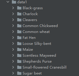
│  ├─Black-grass
│  ├─Charlock
│  ├─Cleavers
│  ├─Common Chickweed
│  ├─Common wheat
│  ├─Fat Hen
│  ├─Loose Silky-bent
│  ├─Maize
│  ├─Scentless Mayweed
│  ├─Shepherds Purse
│  ├─Small-flowered Cranesbill
│  └─Sugar beet
├─mean_std.py
├─makedata.py
├─train.py
├─test1.py
└─test.py

mean_std.py: calculate the values of mean and std.

makedata.py: generate dataset.

Calculate mean and std

In order to make the model converge more quickly, we need to calculate the values of mean and std and create a new mean_std.py, insert code:

from torchvision.datasets import ImageFolder
import torch
from torchvision import transforms

def get_mean_and_std(train_data):
    train_loader = torch.utils.data.DataLoader(
        train_data, batch_size=1, shuffle=False, num_workers=0,
        pin_memory=True)
    mean = torch.zeros(3)
    std = torch.zeros(3)
    for X, _ in train_loader:
        for d in range(3):
            mean[d] += X[:, d, :, :].mean()
            std[d] += X[:, d, :, :].std()
    mean.div_(len(train_data))
    std.div_(len(train_data))
    return list(mean.numpy()), list(std.numpy())


if __name__ == '__main__':
    train_dataset = ImageFolder(root=r'data1', transform=transforms.ToTensor())
    print(get_mean_and_std(train_dataset))

Dataset structure:

Operation results:

([0.3281186, 0.28937867, 0.20702125], [0.09407319, 0.09732835, 0.106712654])

Record this result and use it later!

Generate dataset

The data set structure of our image classification is like this

data
├─Black-grass
├─Charlock
├─Cleavers
├─Common Chickweed
├─Common wheat
├─Fat Hen
├─Loose Silky-bent
├─Maize
├─Scentless Mayweed
├─Shepherds Purse
├─Small-flowered Cranesbill
└─Sugar beet

The default loading method of pytorch and keras is ImageNet dataset format, which is

├─data
│  ├─val
│  │   ├─Black-grass
│  │   ├─Charlock
│  │   ├─Cleavers
│  │   ├─Common Chickweed
│  │   ├─Common wheat
│  │   ├─Fat Hen
│  │   ├─Loose Silky-bent
│  │   ├─Maize
│  │   ├─Scentless Mayweed
│  │   ├─Shepherds Purse
│  │   ├─Small-flowered Cranesbill
│  │   └─Sugar beet
│  └─train
│      ├─Black-grass
│      ├─Charlock
│      ├─Cleavers
│      ├─Common Chickweed
│      ├─Common wheat
│      ├─Fat Hen
│      ├─Loose Silky-bent
│      ├─Maize
│      ├─Scentless Mayweed
│      ├─Shepherds Purse
│      ├─Small-flowered Cranesbill
│      └─Sugar beet

New format conversion script makedata Py, insert code:

import glob
import os
import shutil

image_list=glob.glob('data1/*/*.png')
print(image_list)
file_dir='data'
if os.path.exists(file_dir):
    print('true')
    #os.rmdir(file_dir)
    shutil.rmtree(file_dir)#Delete and re create
    os.makedirs(file_dir)
else:
    os.makedirs(file_dir)

from sklearn.model_selection import train_test_split

trainval_files, val_files = train_test_split(image_list, test_size=0.3, random_state=42)

train_dir='train'
val_dir='val'
train_root=os.path.join(file_dir,train_dir)
val_root=os.path.join(file_dir,val_dir)
for file in trainval_files:
    file_class=file.replace("\\","/").split('/')[-2]
    file_name=file.replace("\\","/").split('/')[-1]
    file_class=os.path.join(train_root,file_class)
    if not os.path.isdir(file_class):
        os.makedirs(file_class)
    shutil.copy(file, file_class + '/' + file_name)

for file in val_files:
    file_class=file.replace("\\","/").split('/')[-2]
    file_name=file.replace("\\","/").split('/')[-1]
    file_class=os.path.join(val_root,file_class)
    if not os.path.isdir(file_class):
        os.makedirs(file_class)
    shutil.copy(file, file_class + '/' + file_name)

Data enhancement Cutout and Mixup

In order to improve my performance, I added two enhancement methods: Cutout and Mixup in the code. To implement these two enhancements, you need to install torch toolbox. Installation command:

pip install torchtoolbox

Cutout is implemented in transforms.

from torchtoolbox.transform import Cutout

# Data preprocessing

transform = transforms.Compose([
    transforms.Resize((224, 224)),
    Cutout()

])

Mixup is implemented in the train method. Need to import package: from Torch toolbox tools import mixup_ data, mixup_ criterion

    for batch_idx, (data, target) in enumerate(train_loader):
        data, target = data.to(device, non_blocking=True), target.to(device, non_blocking=True)
        data, labels_a, labels_b, lam = mixup_data(data, target, alpha)
        optimizer.zero_grad()
        output = model(data)
        loss = mixup_criterion(criterion, output, labels_a, labels_b, lam)
        loss.backward()
        optimizer.step()
        print_loss = loss.data.item()

Import libraries used by the project

import torch.optim as optim
import torch
import torch.nn as nn
import torch.nn.parallel
import torch.utils.data
import torch.utils.data.distributed
import torchvision.transforms as transforms

import torchvision.datasets as datasets
from models.vision_transformer import deit_tiny_patch16_224
from torchtoolbox.tools import mixup_data, mixup_criterion
from torchtoolbox.transform import Cutout

Set global parameters

Set the learning rate, BatchSize, epoch and other parameters to judge whether there is a GPU in the environment. If not, use the CPU. GPU is recommended. The CPU is too slow.

# Set global parameters
modellr = 1e-4
BATCH_SIZE = 16
EPOCHS = 300
DEVICE = torch.device('cuda' if torch.cuda.is_available() else 'cpu')

Image preprocessing and enhancement

Data processing is relatively simple. Cutout, Resize and normalization are added. In transforms Write the values of mean and std obtained above in normalize.

# Data preprocessing
transform = transforms.Compose([
    transforms.Resize((224, 224)),
    Cutout(),
    transforms.ToTensor(),
    transforms.Normalize([0.3281186, 0.28937867, 0.20702125], [0.09407319, 0.09732835, 0.106712654])

])
transform_test = transforms.Compose([
    transforms.Resize((224, 224)),
    transforms.ToTensor(),
    transforms.Normalize([0.3281186, 0.28937867, 0.20702125], [0.09407319, 0.09732835, 0.106712654])
])

Read data

Use pytorch to read the data by default, and then set the dataset_train.class_to_idx is printed out and used for prediction.

# Read data
dataset_train = datasets.ImageFolder('data/train', transform=transform)
dataset_test = datasets.ImageFolder("data/val", transform=transform_test)
print(dataset_train.class_to_idx)
# Import data
train_loader = torch.utils.data.DataLoader(dataset_train, batch_size=BATCH_SIZE, shuffle=True)
test_loader = torch.utils.data.DataLoader(dataset_test, batch_size=BATCH_SIZE, shuffle=False)

class_to_idx results:

{'Black-grass': 0, 'Charlock': 1, 'Cleavers': 2, 'Common Chickweed': 3, 'Common wheat': 4, 'Fat Hen': 5, 'Loose Silky-bent': 6, 'Maize': 7, 'Scentless Mayweed': 8, 'Shepherds Purse': 9, 'Small-flowered Cranesbill': 10, 'Sugar beet': 11}

Set model

• Set the loss function to NN CrossEntropyLoss().
• Set the model to deit_tiny_patch16_224, pre training set to true, num_classes is set to 12.
• The optimizer is set to adam.
• The learning rate adjustment strategy is cosine annealing.

Model file from: https://github.com/rwightman/pytorch-image-models/blob/master/timm/models/vision_transformer.py

I have made changes on the basis of this script, which can be loaded at present pth's pre training model cannot be loaded Pre training model of npz.

# Instantiate the model and move to GPU
criterion = nn.CrossEntropyLoss()
model_ft = deit_tiny_patch16_224(pretrained=True)
print(model_ft)
num_ftrs = model_ft.head.in_features
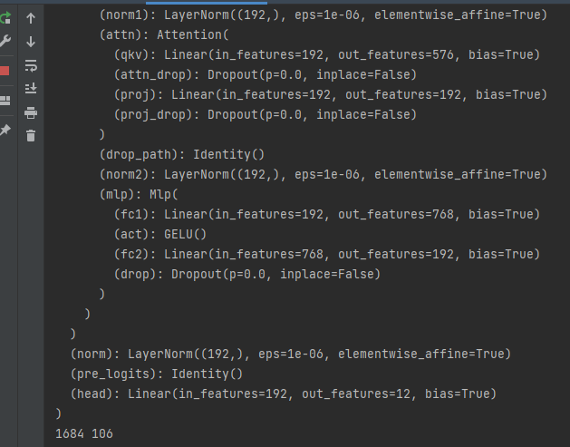
model_ft.head = nn.Linear(num_ftrs, 12,bias=True)
nn.init.xavier_uniform_(model_ft.head.weight)
model_ft.to(DEVICE)
print(model_ft)
# Choose the simple and violent Adam optimizer and lower the learning rate
optimizer = optim.Adam(model_ft.parameters(), lr=modellr)
cosine_schedule = optim.lr_scheduler.CosineAnnealingLR(optimizer=optimizer,T_max=20,eta_min=1e-9)

Define training and verification functions

# Define training process
alpha=0.2
def train(model, device, train_loader, optimizer, epoch):
    model.train()
    sum_loss = 0
    total_num = len(train_loader.dataset)
    print(total_num, len(train_loader))
    for batch_idx, (data, target) in enumerate(train_loader):
        data, target = data.to(device, non_blocking=True), target.to(device, non_blocking=True)
        data, labels_a, labels_b, lam = mixup_data(data, target, alpha)
        optimizer.zero_grad()
        output = model(data)
        loss = mixup_criterion(criterion, output, labels_a, labels_b, lam)
        loss.backward()
        optimizer.step()
        lr = optimizer.state_dict()['param_groups'][0]['lr']
        print_loss = loss.data.item()
        sum_loss += print_loss
        if (batch_idx + 1) % 10 == 0:
            print('Train Epoch: {} [{}/{} ({:.0f}%)]\tLoss: {:.6f}\tLR:{:.9f}'.format(
                epoch, (batch_idx + 1) * len(data), len(train_loader.dataset),
                       100. * (batch_idx + 1) / len(train_loader), loss.item(),lr))
    ave_loss = sum_loss / len(train_loader)
    print('epoch:{},loss:{}'.format(epoch, ave_loss))

ACC=0
# Verification process
def val(model, device, test_loader):
    global ACC
    model.eval()
    test_loss = 0
    correct = 0
    total_num = len(test_loader.dataset)
    print(total_num, len(test_loader))
    with torch.no_grad():
        for data, target in test_loader:
            data, target = Variable(data).to(device), Variable(target).to(device)
            output = model(data)
            loss = criterion(output, target)
            _, pred = torch.max(output.data, 1)
            correct += torch.sum(pred == target)
            print_loss = loss.data.item()
            test_loss += print_loss
        correct = correct.data.item()
        acc = correct / total_num
        avgloss = test_loss / len(test_loader)
        print('\nVal set: Average loss: {:.4f}, Accuracy: {}/{} ({:.0f}%)\n'.format(
            avgloss, correct, len(test_loader.dataset), 100 * acc))
        if acc > ACC:
            torch.save(model_ft, 'model_' + str(epoch) + '_' + str(round(acc, 3)) + '.pth')
            ACC = acc


# train

for epoch in range(1, EPOCHS + 1):
    train(model_ft, DEVICE, train_loader, optimizer, epoch)
    cosine_schedule.step()
    val(model_ft, DEVICE, test_loader)

Operation results:

test

We introduce a general method to manually load data sets and then make predictions. The specific operations are as follows:

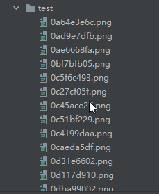
The directory where the test set is stored is shown in the following figure:

The first step is to define the category. The order of this category corresponds to the category order during training. Do not change the order!!!!

The second step is to define transforms, which is the same as the transforms of the verification set, without data enhancement.

Step 3: load the model and put it in DEVICE,

Step 4: read the picture and predict the category of the picture. Here, note that the Image of PIL library is used to read the picture. Don't use cv2. transforms doesn't support it.

import torch.utils.data.distributed
import torchvision.transforms as transforms
from PIL import Image
from torch.autograd import Variable
import os
classes = ('Black-grass', 'Charlock', 'Cleavers', 'Common Chickweed',
           'Common wheat','Fat Hen', 'Loose Silky-bent',
           'Maize','Scentless Mayweed','Shepherds Purse','Small-flowered Cranesbill','Sugar beet')
transform_test = transforms.Compose([
         transforms.Resize((224, 224)),
        transforms.ToTensor(),
        transforms.Normalize([0.3281186, 0.28937867, 0.20702125], [0.09407319, 0.09732835, 0.106712654])
])
 
DEVICE = torch.device("cuda:0" if torch.cuda.is_available() else "cpu")
model = torch.load("model.pth")
model.eval()
model.to(DEVICE)
 
path='test/'
testList=os.listdir(path)
for file in testList:
        img=Image.open(path+file)
        img=transform_test(img)
        img.unsqueeze_(0)
        img = Variable(img).to(DEVICE)
        out=model(img)
        # Predict
        _, pred = torch.max(out.data, 1)
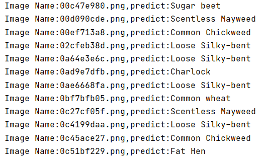
        print('Image Name:{},predict:{}'.format(file,classes[pred.data.item()]))

Operation results: