From Excel to Python: the most commonly used 36 Pandas functions
About Excel, you must use 36 Python functions
This paper deals with the 36 most commonly used functions of pandas. Through these functions, it introduces how to complete data generation and import, data cleaning, preprocessing, as well as the most common data classification, data filtering, classification summary, perspective and other most common operations.
Generate data table
There are two common methods to generate data tables, the first is to import external data, and the second is to write data directly.
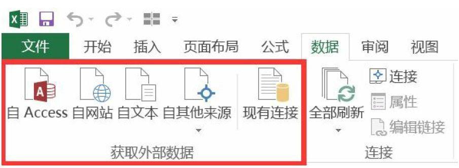
The "file" menu in Excel provides the function of obtaining external data, and supports the import of multiple data sources of database, text file and page.
Python supports importing from multiple types of data. You need to import numpy and pandas libraries before you start to import data in Python
import numpy as np
import pandas as pd
Import external data
df=pd.DataFrame(pd.read_csv('name.csv',header=1))
df=pd.DataFrame(pd.read_Excel('name.xlsx'))c
There are many optional parameter settings, such as column name, index column, data format, etc
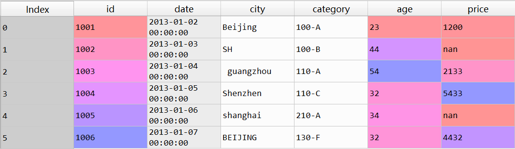
Write data directly
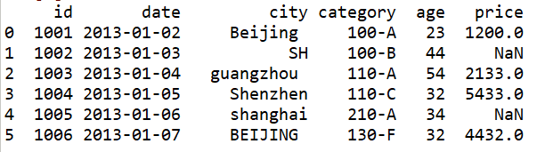
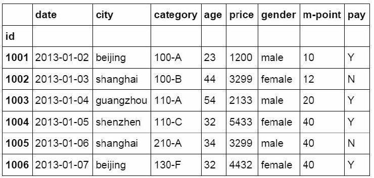
df = pd.DataFrame({"id":[1001,1002,1003,1004,1005,1006],
"date":pd.date_range('20130102', periods=6),
"city":['Beijing ', 'SH', ' guangzhou ', 'Shen
zhen', 'shanghai', 'BEIJING '],
"age":[23,44,54,32,34,32],
"category":['100-A','100-B','110-A','110-C','2
10-A','130-F'],
"price":[1200,np.nan,2133,5433,np.nan,4432]},
columns =['id','date','city','category','age',
'price'])
Data sheet check
The purpose of data table inspection is to understand the overall situation of the data table, obtain the key information and data overview of the data table, such as the size, occupied space, data format, whether there are empty values, duplicates and specific data content of the whole data table, so as to prepare for the subsequent cleaning and pretreatment.
1. Data dimension (row and column)
You can view row and column numbers in Excel by using CTRL + down cursor keys and CTRL + right cursor keys. In Python, the shape function is used to view the dimensions of the data table, that is, the number of rows and columns.
df.shape
2. Data sheet information
Use the info function to view the overall information of the data table, including data dimension, column name, data format and occupied space. #Data sheet information
df.info()
<class 'pandas.core.frame.DataFrame'>
RangeIndex: 6 entries, 0 to 5
Data columns (total 6 columns):
id 6 non-null int64
date 6 non-null datetime64[ns]
city 6 non-null object
category 6 non-null object
age 6 non-null int64
price 4 non-null float64
dtypes: datetime64[ns](1), float64(1), int64(2), object(2)
memory usage: 368.0+ bytes
3. View data format
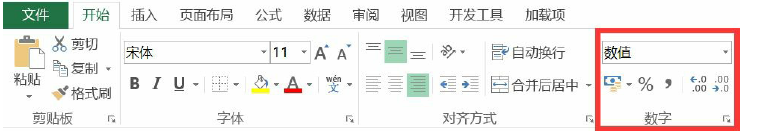
Excel determines the format of data by selecting cells and viewing the value types in the start menu. The dtypes function is used in Python to return the data format.
Dtypes is a function for viewing data formats. You can view all data formats in a data table at once, or you can specify a column to view separately
#View data table column formats
df.dtypes
id int64
date datetime64[ns]
city object
category object
age int64
price float64
dtype: object
#View single column format
df['B'].dtype
dtype('int64')
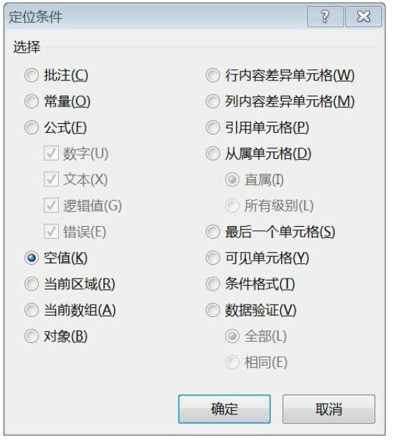
4. View null value
The way to view null values in Excel is to use "find and select" directory under "start" directory with "positioning conditions"
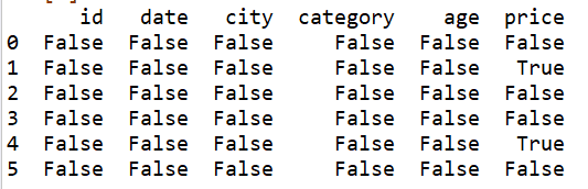
Isnull is a function that checks for null values in Python
#Check data null
df.isnull()
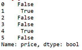
#Check for specific column nulls
df['price'].isnull()
5. View unique value
The way to view unique values in Excel is to color them using conditional formatting.
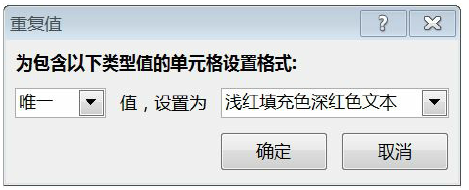
Use the unique function in Python to view unique values.
#View unique values in the city column
df['city'].unique()
array(['Beijing ', 'SH', ' guangzhou ', 'Shenzhen', 'shanghai', '
BEIJING '], dtype=object)
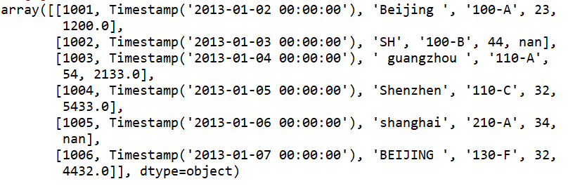
6. View data table values
The Values function in Python is used to view the Values in the data table
#View values of data table
df.values
7. View column name
The colors function is used to view the column names in the data table separately.
#View column name
df.columns
Index(['id', 'date', 'city', 'category', 'age', 'price'], dtype='
object')
8. View the first 10 rows of data
The Head function is used to view the first N rows of data in the data table
#View the first three rows of data
df.head(3)
9. View the last 10 rows of data
The number of Tail rows is the opposite of the head function, which is used to view the data of the last N rows in the data table
#View last 3 lines
df.tail(3)
Data sheet cleaning
This chapter introduces how to clean the problems in the data table, including the handling of null value, case problem, data format and duplicate value.
1. Process null values (delete or fill)
Null values can be processed through find and replace function in Excel
The method of handling null values in Python is flexible. You can use Dropna function to delete the data with null values in the data table, or use fillna function to fill in null values.
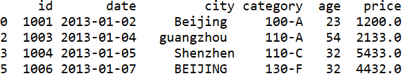
#Delete rows with null values in the data table
df.dropna(how='any')
You can also use numbers to fill in null values
#Fill the data table with the number 0
df.fillna(value=0)
Use the mean value of the price column to fill in the NA field. Also use the fillna function. Use the mean function in the value to be filled to calculate the current mean value of the price column, and then use the mean value to fill in the NA field.
#useprice Mean pairNA Fill in
df['price'].fillna(df['price'].mean())
Out[8]:
0    1200.0
1    3299.5
2    2133.0
3    5433.0
4    3299.5
5    4432.0
Name: price, dtype: float64
2. Clear space
Space in character is also a common problem in data cleaning
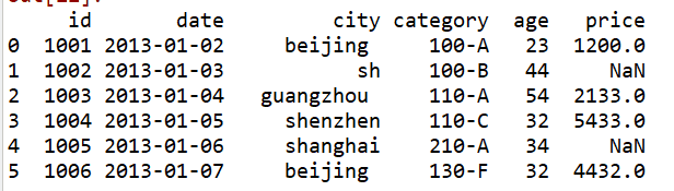
#Clear character spaces in city fields
df['city']=df['city'].map(str.strip)
3. Case conversion
In English fields, it is also a common problem that the case of letters is not uniform. Excel has functions such as UPPER and LOWER. Python also has functions with the same name to solve case problems.
#city column case conversion
df['city']=df['city'].str.lower()
4. Change data format
The data format can be modified in Excel through the format cell function.
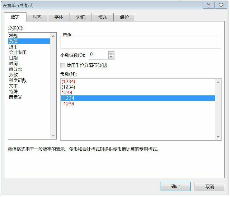
In Python, the astype function is used to modify the data format.
#Change data format
df['price'].astype('int')
0 1200
1 3299
2 2133
3 5433
4 3299
5 4432
Name: price, dtype: int32
5. Change column name
Rename is a function to change the column name. We will change the category column in the data table to category size in the future.
#Change column name
df.rename(columns={'category': 'category-size'})
6. Delete duplicate values
Excel data directory has the function of "delete duplicates"

Delete duplicate values in Python using the drop? Duplicates function
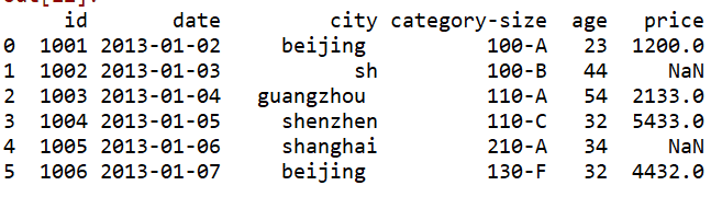
df['city']
0 beijing
1 sh
2 guangzhou
3 shenzhen
4 shanghai
5 beijing
Name: city, dtype: object
There are duplicates in the city column, which are deleted in the first and last drop ABCD duplicates() functions respectively
#Duplicate values after deletion
df['city'].drop_duplicates()
0 beijing
1 sh
2 guangzhou
3 shenzhen
4 shanghai
Name: city, dtype: object
After setting the keep='last 'parameter, in contrast to the previous result of deleting duplicate values, the first occurrence of beijing is deleted
#Delete previous duplicate values
df['city'].drop_duplicates(keep='last')
1 sh
2 guangzhou
3 shenzhen
4 shanghai
5 beijing
Name: city, dtype: objec
7. Value modification and replacement
Using "find and replace" function in Excel can realize the replacement of numerical value

Using replace function to realize data replacement in Python
#Data replacement
df['city'].replace('sh', 'shanghai')
0 beijing
1 shanghai
2 guangzhou
3 shenzhen
4 shanghai
5 beijing
Name: city, dtype: object
Data preprocessing
This chapter mainly deals with data preprocessing, sorting out the cleaned data for later statistics and analysis. It mainly includes data table merging, sorting, numerical value sorting, data grouping and marking.
1. Data table consolidation
There is no function of data table merging in Excel, which can be realized step by step by VLOOKUP function. In Python, it can be implemented at one time through the merge function.
#Establish df1 data table
df1=pd.DataFrame({"id":[1001,1002,1003,1004,1005,1006,1007,1008],
"gender":['male','female','male','female','male
','female','male','female'],
"pay":['Y','N','Y','Y','N','Y','N','Y',],
"m-point":[10,12,20,40,40,40,30,20]})
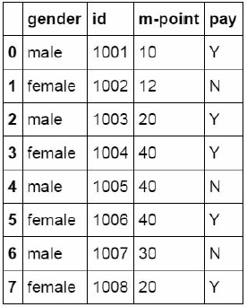
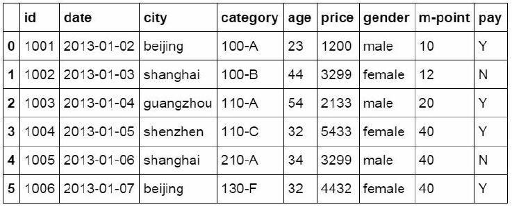
The merge function is used to merge the two data tables. The merge method is inner, which matches the data shared by the two data tables together to generate a new data table. And it is named DF ﹣ inner.
#Data table match merge
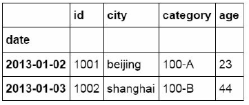
df_inner=pd.merge(df,df1,how='inner')
There are also left, right and outer ways to merge
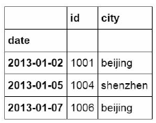
df_left=pd.merge(df,df1,how='left')
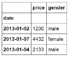
df_right=pd.merge(df,df1,how='right')
df_outer=pd.merge(df,df1,how='outer')
2. Set index column
Index column can be used for data extraction, summary and data filtering
#Set index column
df_inner.set_index('id')
3. Sort (by index, by value)
In Excel, you can sort the data table directly through the sort button in the data directory
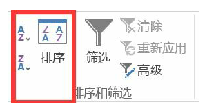
In Python, you need to use the ort_values function and sort_index function to complete sorting
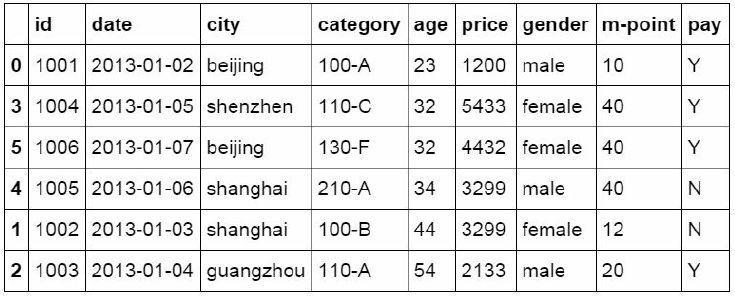
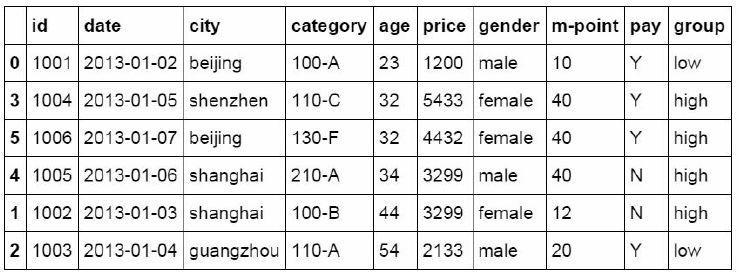
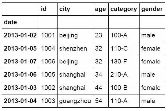
#Sort by value of a specific column
df_inner.sort_values(by=['age'])
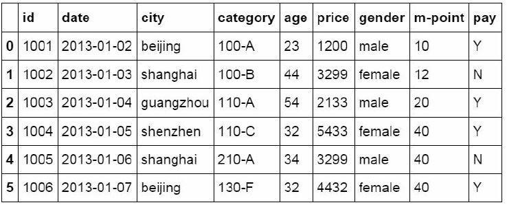
The sort? Index function is used to sort the data table by the value of the index column.
#Sort by index column
df_inner.sort_index()
4. Data grouping
In Excel, you can use the VLOOKUP function to perform approximate matching to complete grouping of values, or use the PivotTable to complete grouping
Where function is used to judge and group data in Python
#If the price column's value is > 3000, the group column shows high, otherwise low
df_inner['group'] = np.where(df_inner['price'] > 3000,'high','low
')
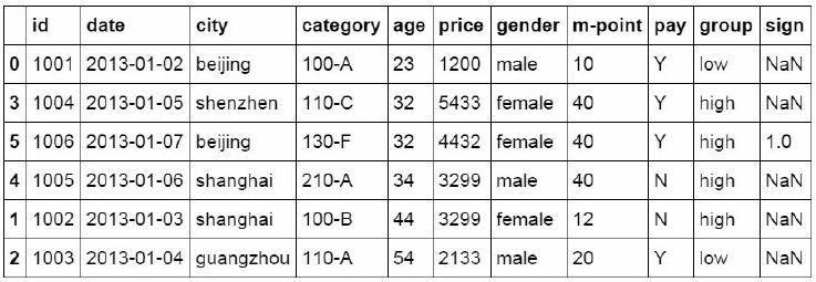
You can also group data after judging the values of multiple fields. In the following code, the data with city column equal to beijing and price column greater than or equal to 4000 is marked as 1.
#Group data with multiple conditions
df_inner.loc[(df_inner['city'] == 'beijing') & (df_inner['price']
>= 4000), 'sign']=1
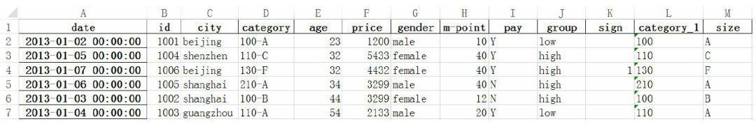
5. Data breakdown
"Column" function is provided under the data directory in Excel.

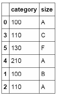
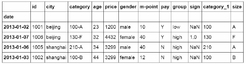
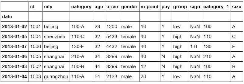
In Python, we use the split function to realize that the data listed in the category column of the data table contains two information. The first number is the category id, and the last letter is the size value. The middle is hyphenated. We use the split function to split this field and match the split data table back to the original data table.
#The values of the category field are listed in turn, and a data table is created. The index value is the index column of df_inner, and the column name is called category and size
pd.DataFrame((x.split('-') for x in df_inner['category']),index=d
f_inner.index,columns=['category','size'])
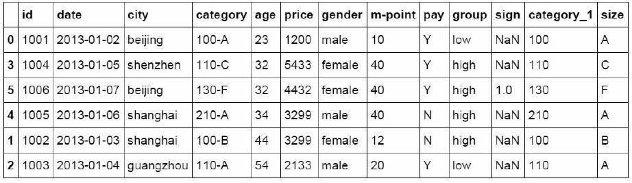
#Match the completed data table with the original DF ﹣ inner data table
df_inner=pd.merge(df_inner,split,right_index=True, left_index=Tru
e)
Data extraction
1. Extract by label (loc)
#Extract the value of a single row by index
df_inner.loc[3]
id 1004
date 2013-01-05 00:00:00
city shenzhen
category 110-C
age 32
price 5433
gender female
m-point 40
pay Y
group high
sign NaN
category_1 110
size C
Name: 3, dtype: object
Use colons to limit the range of extracted data, preceded by the start tag value and followed by the end tag value.
#Extract area row values by index
df_inner.loc[0:5]
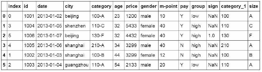
The reset? Index function is used to recover the index. Here, we reset the date of the date field to the index of the data table, and extract the data according to the date.
#Reset index
df_inner.reset_index()
#Set date as index
df_inner=df_inner.set_index('date')
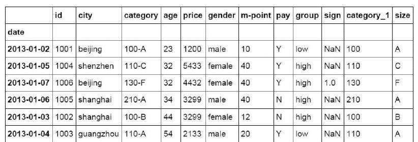
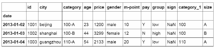
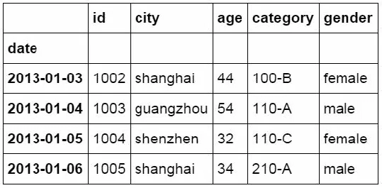
#Extract all data before 4 days
df_inner[:'2013-01-04']
2. Extraction by location (iloc)
Use the iloc function to extract the data in the data table by location. The number before and after the colon is no longer the label name of the index, but the location of the data, starting from 0.
#useiloc Extract data by location area
df_inner.iloc[:3,:2]
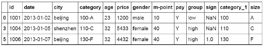
In addition to extracting data by region, iloc function can also extract data by location one by one
#useiloc Extract data individually by location
df_inner.iloc[[0,2,5],[4,5]]
The 0,2,5 in the square brackets at the front represents the position of the row where the data is located, and the number in the square brackets at the back represents the position of the column where the data is located.
3. Extract by label and location (ix)
ix is a mixture of loc and iloc, which can extract data by index tag and location
#Using ix to extract data by index label and location
df_inner.ix[:'2013-01-03',:4]
4. Extract by condition (area and condition value)
Use the two functions of loc and isin to extract data according to specified conditions
#Determine whether the value of the city column is beijing
df_inner['city'].isin(['beijing'])
date
2013-01-02 True
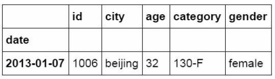
2013-01-05 False
2013-01-07 True
2013-01-06 False
2013-01-03 False
2013-01-04 False
Name: city, dtype: bool
The isin function is nested in the data extraction function of loc, and the result is extracted as the Ture data. Here we change the judgment condition to whether the city value is beijing and shanghai. If so, extract this data.
#First, determine whether the city column contains beijing and shanghai, and then extract the data of composite conditions.
df_inner.loc[df_inner['city'].isin(['beijing','shanghai'])]
Data filtering
Filter by criteria (and, or, not)
The "filter" function is provided under the Excel data directory, which is used to filter the data table according to different conditions.
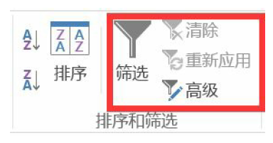
In Python, the loc function is used in conjunction with the filter criteria to complete the filtering function. With sum and count functions, the functions of sumif and counttif in Excel can also be realized. Use the and condition to filter if you are older than 25 and the city is beijing.
#Filter with and criteria
df_inner.loc[(df_inner['age'] > 25) & (df_inner['city'] == 'beiji
ng'), ['id','city','age','category','gender']]/
#Filter with or criteria
df_inner.loc[(df_inner['age'] > 25) | (df_inner['city'] == 'beiji
ng'), ['id','city','age','category','gender']].sort(['age'])
#Filter with non criteria
df_inner.loc[(df_inner['city'] != 'beijing'), ['id','city','age',
'category','gender']].sort(['id'])
Add the city column after the previous code and use the count function to count. Function equivalent to countifs function in Excel
#Count the filtered data by city column
df_inner.loc[(df_inner['city'] != 'beijing'), ['id','city','age',
'category','gender']].sort(['id']).city.count()
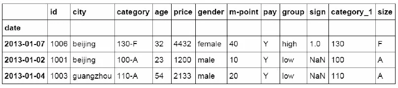
Another way to filter is to use the query function
#Filter using the query function
df_inner.query('city == ["beijing", "shanghai"]')

Add the price field and sum function after the previous code. Sum the filtered price field, which is equivalent to the function of sumifs in Excel.
#Sum the filtered results by price
df_inner.query('city == ["beijing", "shanghai"]').price.sum()
12230
Data summary
Excel uses subtotal and pivoting to summarize data by specific dimensions. The main functions used in Python are groupby and pivot table.
1. Classification and summary
#Count all columns
df_inner.groupby('city').count()/
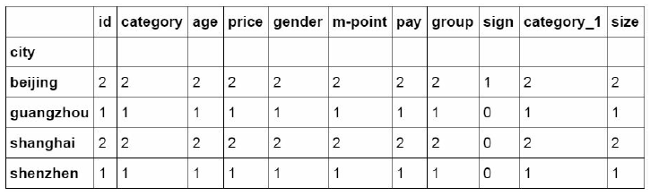
#Count and summarize specific ID columns
df_inner.groupby('city')['id'].count()
city
beijing 2
guangzhou 1
shanghai 2
shenzhen 1
Name: id, dtype: int64
#Summarize and count the two fields
df_inner.groupby(['city','size'])['id'].count()
city size
beijing A 1
F 1
guangzhou A 1
shanghai A 1
B 1
shenzhen C 1
Name: id, dtype: int64
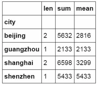
You can also calculate the summarized data by multiple dimensions at the same time
#Summarize the city field and calculate the total and average value of price.
df_inner.groupby('city')['price'].agg([len,np.sum, np.mean])
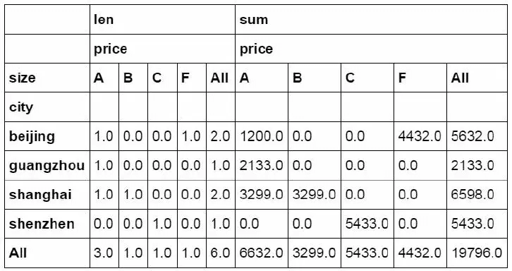
2. Data perspective

In Python, the same effect is achieved through the pivot table function
#Set city as the row field, size as the column field, and price as the value field.
The quantity and amount of price are calculated separately and summarized by rows and columns.
pd.pivot_table(df_inner,index=["city"],values=["price"],columns=[
"size"],aggfunc=[len,np.sum],fill_value=0,margins=True)
data statistics
1. Data sampling
The data sampling function is provided in the data analysis function of Excel

Python completes data sampling through the sample function
#Simple data sampling
df_inner.sample(n=3)
The Weights parameter is the weight of the sampling. You can change the result of the sampling by setting different Weights
#Set sampling weight manually
weights = [0, 0, 0, 0, 0.5, 0.5]
df_inner.sample(n=2, weights=weights)
The parameter replace in the Sample function is used to set whether to put it back after sampling
#Do not put back after sampling
df_inner.sample(n=6, replace=False)
#Put it back after sampling
df_inner.sample(n=6, replace=True)
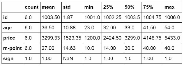
2. Descriptive statistics
Data can be described and counted through description in Python
#Descriptive statistics of data table
df_inner.describe().round(2).T
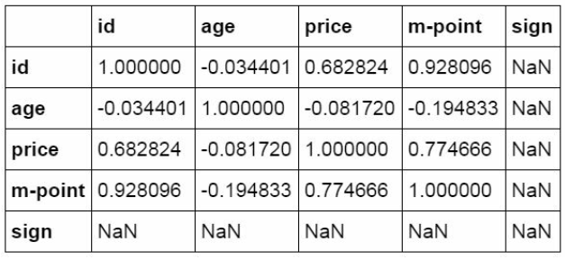
3. Correlation analysis
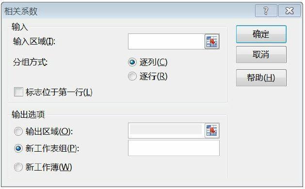
In Python, the corr function completes the operation of correlation analysis and returns the correlation coefficient.
#correlation analysis
df_inner['price'].corr(df_inner['m-point'])
0.77466555617085264
#Data table correlation analysis
df_inner.corr()
data output
1. Write to Excel
#Export to Excel format
df_inner.to_Excel('Excel_to_Python.xlsx', sheet_name='bluewhale_c
c')
2. Write csv
#Export to CSV format
df_inner.to_csv('Excel_to_Python.csv')
#In the process of learning Python, I often don't want to learn it because there is no information or guidance, so I specially prepared a group of 592539176. There are a large number of PDF books and tutorials in the group for free use! No matter which stage you learn, you can get the corresponding information!
Reference resources
From Excel to Python: an advanced guide to data analysis