Project Background

The current situation of the problem: improving the low activation rate and first charge rate KPI of China Telecom Card;
Technical selectivity: python completes data cleaning and model training, PowerBI builds dynamic dashboard;
Project Profile:
(1) Each row of the data set describes the detailed user information, card information and logistic signing information of purchasing China Telecom Card; (2) Our goal is to establish training model based on the information data of inputted purchasing card users, to predict the activation rate and the first charge rate of all kinds of cards; (3) to draw sub-regions and sub-years. User portraits of card purchasing groups under the age group, analysis of consumer habits and card purchasing preferences, to achieve targeted promotion; (4) Based on Logistics track tracking, in-depth mining, analysis of user activation, first charge failure reasons, help China Telecom to enhance the activation rate and first charge rate of card products.

The whole process of data analysis/mining

Data cleaning

Identity Card Coding Rules:
There are 18 new Chinese ID cards. Among them, the first 17 bits are information codes, and the last one is check codes. Each bit of information codes can be 0-9 digits, while check codes can be 0-9 or X, where X represents 10.
Numbers 1-2 denote "location identity (or autonomous region, municipality directly under the Central Government)"; numbers 3-4 denote "city (or state)"; numbers 5-6 denote "county (or county-level city)"; the top two of the last four denote "number of local police station"; numbers 4 and 17 denote "gender", and odd. Number is "male" and even number is "female".

Demo

# Import Library
import pandas as pd
import numpy as np
import re
import os
import datetime
 print('Import Successful')
pd.set_option('display.max_columns',200)
pd.set_option('max_row',200)
pd.set_option("display.float_format", lambda x: "%.2f" % x)
# Read in data
 DF = pd. read_excel (r'D: 000-mine Richang 2019 temporary 0719 order details. xlsx', SEP =  t', index_col = None)
>>>df.info()
<class 'pandas.core.frame.DataFrame'>
RangeIndex: 217589 entries, 0 to 217588
Data columns (total 95 columns):
Order number 217589 non-null object
 Original order 217589 non-null object
 Order type 217589 non-null object
 Order status 217589 non-null object
 Order sub-state 69050 non-null object
 Cancellation reason 4 non-null object
 Order pending cause 3834 non-null object
 Installation Failure Cause 0 non-null float64
 Order source 217589 non-null object
 Settlement status 0 non-null float64
 Payment Platform 217589 non-null object
 Price 0 non-null float64
 Shop 217589 non-null object
 AB type 217589 non-null object
 Split type 217589 non-null object
 System type 217589 non-null object
 Order amount 217589 non-null float64
 Payment method 217589 non-null object
 Payment Pipeline No. 2930 non-null object
 Collection of Card No. 0 non-null float64
 Order generation time 217589 non-null object
 Payment completion time 2995 non-null object
 Transaction completion time 119861 non-null object
 Delivery time 163250 non-null object
 Logistics sheet backfilling time 7 non-null object
 User name 4426 non-null object
 QQ No. 0 non-null float64
 User name 215737 non-null object
 Access ID No. 215737 non-null object
 Access mobile phone number 217589 non-null int64
 Contact number 69455 non-null object
ICCID          0 non-null float64
 Contact address 196568 non-null object
 Name of consignee 217589 non-null object
 Receiving address 217589 non-null object
 The consignee's telephone number 217589 non-null object
 Consignee mailbox 861 non-null object
 Zip code 152436 non-null float64
 217589 non-null object in province/city/county
 0 non-null float64 in the province/city/county where the netizens live
 No. 217589 non-null object
 Distribution mode 70269 non-null object
 Business hall address 0 non-null float64
 Distribution time 810 non-null object
 Preferential voucher 0 non-null float64
 Coupon code 0 non-null float64
 F code 0 non-null float64
 F code name 0 non-null float64
 Product Recommender 14 non-null object
 CPS Recommender 212761 non-null object
 Order Note 10338 non-null object
 Logistics No. 162756 non-null object
 Logistics signing time 75132 non-null object
 Carrier 163250 non-null object
 Whether to upload and sign certificate 217589 non-null object
 Advance Deposit Invoice Category 147439 non-null object
 Goods invoice payable to 147320 non-null object
 Item Fee Heading Name 145422 non-null object
 Invoice content 147439 non-null object
 Enterprise Tax No. 0 non-null float64
 User message 48 non-null object
 Size card type 182231 non-null object
 Card writing channel 217589 non-null int64
 Card number 68 non-null float64
 Serial number 0 non-null float64
 Sales No. 217589 non-null int64
 Sales Name 217589 non-null object
 Sales Type 217589 non-null object
 Sales volume 0 non-null float64
 Sales price 0 non-null float64
 Partner 0 non-null float64
 Actual amounting of 0 non-null float64
 Package 217589 non-null object
 Main number 217589 non-null int64
 Sub-number 1327 non-null float64
 Cash advance deposit 246 non-null object
 Optional package 1327 non-null object
 Contract subsidy 0 non-null float64
 Other 0 non-null float64
 Beautiful signal low elimination 214485 non-null float64
 Beauty grade 214485 non-null float64
 Beautiful Advance Deposit 214485 non-null float64
 Business hall delivery mode 151962 non-null object
 Is offline mode 151962 non-null object
 Whether to turn off line 39313 non-null object
 Reasons for offline turnaround 39313 non-null object
 Business hall delivery iccid 143252 non-null float64
 Identity card picture 1 137987 non-null object
 Identity card picture 2 136009 non-null object
 Identity card picture 3 135960 non-null object
 Identity card picture 4 135960 non-null object
 Time 0 non-null float64 in real-name Information Review
 Sales text step name 0 non-null float64
 User-selected step content 0 non-null float64
 Reasons for inaccessibility of Jingdong 21079 non-null object
dtypes: float64(31), int64(4), object(60)
memory usage: 157.7+ MB

Screening valid column data for analysis of "user activation" and data cleaning

sf_df=pd.DataFrame(df,index=df.index,columns=['Order Number','Order status','Order generation time','Logistics Document Number','Transaction completion time','User Name','Access ID number','Access Mobile Number','Consignee Name','Province / city / county','Number Attribution','Sales No.','Sales Name'])
sf_df.dropna(subset=['Access ID number'],inplace=True)  #Delete empty line data with "Access ID Card Number"
sf_df.reset_index(drop=True,inplace=True)   #Reset the index and delete the original index

# (1) According to the difference between "order generation time" and "transaction completion time", i.e. the "transaction cycle" column, the time difference is changed to "hour". If the time difference is changed to "day", it is enough to replace h with D:
sf_df['Transaction cycle']=pd.DataFrame((pd.to_datetime(sf_df['Transaction completion time'])-pd.to_datetime(sf_df['Order generation time'])).values/np.timedelta64(1,'h'))    #Time in Dataframe can not be added or subtracted directly, so we need to use pandas to_datetime() method to convert it into time format for addition and subtraction, and then into df format.

# (2) Sex extraction based on ID number
sf_df['Gender']=sf_df['Access ID number'].str.slice(16,17)
sf_df['Gender'] = pd.to_numeric(sf_df['Gender'])   #This function converts object to numerical form
def get_sex(str1):
    #Check Gender
    if str1 % 2 ==0:
        return 'female'
    else:
        return 'male'

sf_df['Gender'] =  sf_df['Gender'].apply(get_sex)

# (3) Classifying users according to age
sf_df['Age'] =sf_df['Access ID number'].str.slice(6,10)   #Extracting "Age Information" from "Access ID Card Number"
sf_df['Age']=pd.to_numeric(sf_df['Age'])  ##This function converts object to numerical form
# print(sf_df.loc[:10, ['age classification'])
now_year=pd.datetime.now().year  #Get the current year
# print("The current time is:", now_year)
sf_df['Age']=now_year-sf_df['Age']  #Current Year - Birth Age Obtained, Age Classification
# print(sf_df.loc[:10, ['age classification'])
def get_year_group(str1):  #Defining Age Classification Function
    if str1 <= 18:
        return "juvenile"
    elif str1 < 30:
        return "Weak crown"
    elif str1 < 40:
        return "While standing"
    elif str1 < 50:
        return "Not puzzled"
    elif str1 < 60:
        return "Know destiny"
    elif str1 < 70:
        return "Flower armor"
    else:
        return "old age"

sf_df['Age classification']=sf_df['Age'].apply(get_year_group)  #Call the age grading function and use df[col_name].apply(function_name)

# (4)take'Number Attribution'The columns of "Number Ownership Province" and "Number Ownership City" are divided into two columns.   #That is to say, to analyze the user's regional characteristics
df_add=pd.DataFrame((x.split('/') for x in sf_df['Number Attribution']),
                    index=sf_df.index,columns=['Number Ownership Province','Number Ownership City'])
sf_df=sf_df.join(df_add)
sf_df.drop(['Number Attribution'],axis=1,inplace=True)

# (5) Screening the order of "order and activation quantity of delivery". Provisions: "Delivery" is "Logistics Order Number" is not empty orders, "Activation" is "Order Status" is "Transaction Completed" orders.
sf_df_fahuo=sf_df[sf_df['Logistics Document Number'].notnull()]   #Screening out the line data that "Logistics Document Number" is not empty, that is, "Delivery Quantity"

# (6) Add the column "Activated or Not", assign 1 for "Activated Order" and 0 for "Activated Order" according to "Order Status" as "Transaction Completed";
sf_df_fahuo['Activation or not']=None
def jh_decide(str1):
    if(str1=="Completion of the transaction"):
        return 1
    else:
        return 0
    
sf_df_fahuo['Activation or not']=sf_df_fahuo['Order status'].apply(jh_decide)
# print(sf_df_fahuo.loc[:100,['Order status','Activation or not']])   #Verify that the new column "Activated or Not" corresponds to "Order Status"

The order data of "delivery volume" are obtained, and the next step is to match the "product label card".

#Matching product label card
biaoka=pd.read_excel(r'D:\000-mine\richang2019\Raw Data Set\Product Standard Card 0709.xlsx',sep='\t',index_col=None)
biaoka.drop_duplicates(subset=['Sales No.'],keep='last',inplace=True)  #Duplicate removal
biaoka.drop(['Sales Name'],axis=1,inplace=True)
sf_df_fahuo=pd.merge(sf_df_fahuo,biaoka,how='left',on='Sales No.')
print(biaoka.info())
>>>
<class 'pandas.core.frame.DataFrame'>
Int64Index: 668 entries, 34 to 706
Data columns (total 2 columns):
//Sales No.    668 non-null int64
//Product Classification     668 non-null object
dtypes: int64(1), object(1)

The preliminary data cleaning is over. The next step is data analysis.

Data analysis

Part01: Characteristic correlation analysis and calculation
The relationship between "activation or not" and the characteristic variables of "gender", "age classification", "product classification", "number ownership province", "transaction cycle" was analyzed.

#Feature correlation analysis, spearman for discrete variables
print(sf_df_fahuo['Activation or not'].corr(sf_df_fahuo['Gender'],method='spearman'))  #Calculation of correlation between two columns
print(sf_df_fahuo['Activation or not'].corr(sf_df_fahuo['Age classification'],method='spearman')) 
print(sf_df_fahuo['Activation or not'].corr(sf_df_fahuo['Number Ownership Province'],method='spearman')) 
print(sf_df_fahuo['Activation or not'].corr(sf_df_fahuo['Product Classification'],method='spearman'))
print(sf_df_fahuo['Activation or not'].corr(sf_df_fahuo['Transaction cycle'],method='spearman'))
print("="*50)
print(sf_df_fahuo['Product Classification'].corr(sf_df_fahuo['Gender'],method='spearman'))
print(sf_df_fahuo['Product Classification'].corr(sf_df_fahuo['Age classification'],method='spearman'))
print(sf_df_fahuo['Product Classification'].corr(sf_df_fahuo['Number Ownership Province'],method='spearman'))
print(sf_df_fahuo['Product Classification'].corr(sf_df_fahuo['Transaction cycle'],method='spearman'))
>>>
-0.07506799907748103
0.13565676413724592
0.0029258613799464737
-0.14785852579925973
-0.004775989850378669
==================================================
0.13259535769556047
-0.17013142844828066
-0.008068636413560124
0.6001361002699821

Part02: Visual Analysis of Data
Analysis of the Relationships among Characteristic Variables from Different Dimensions

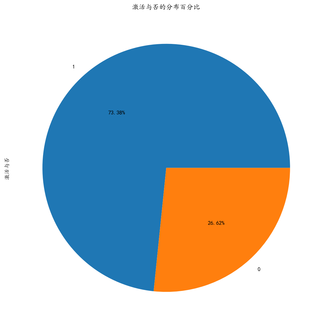
# Import a database for data visualization
import matplotlib.pyplot as plt
import seaborn as sns
%config InlineBackend.figure_format='retina'  #Display HD pictures on the screen
%matplotlib inline     #image display
import matplotlib as mpl            #Solving the problem of Chinese non-recognition
import matplotlib.ticker as ticker
mpl.rcParams['font.sans-serif']=['KaiTi']  
mpl.rcParams['font.serif']=['KaiTi']
mpl.rcParams['axes.unicode_minus']=False  # Solve the problem of saving an image as a negative sign'-'displayed as a box, or converting a negative sign to a string

#Overall Distribution of "Activated or Not" Order -- "1" means "Activated" and "0" means "Unactivated"
f,ax=plt.subplots(1,1,figsize=(10,10))
sf_df_fahuo['Activation or not'].value_counts().plot.pie(autopct='%1.2f%%')
ax.set_title("Percentage distribution of activation or inactivation")

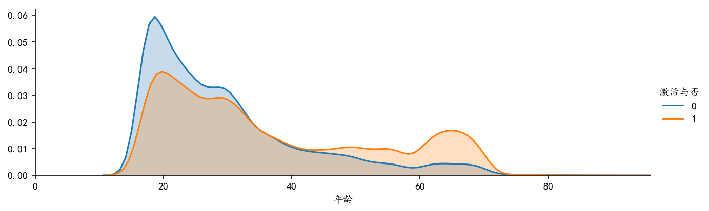
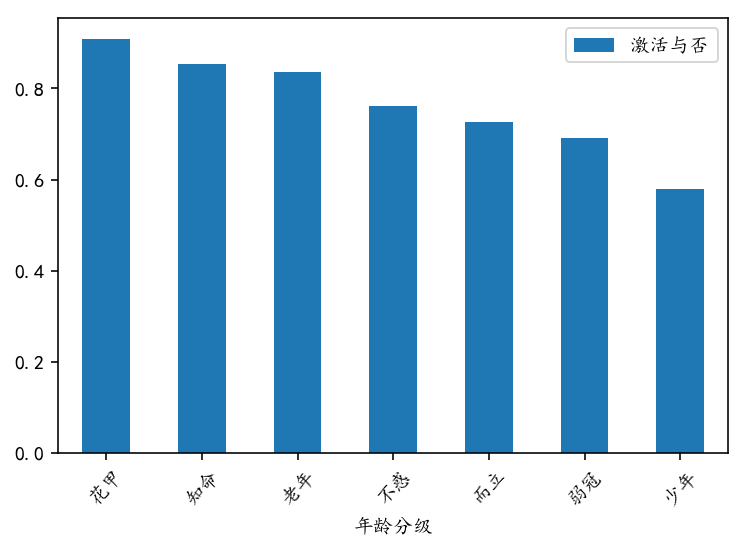
#Distribution of different age groups
print(sf_df_fahuo['Age'].describe()) 
>>>
count   162756.00
mean        34.76
std         15.87
min         15.00
25%         22.00
50%         30.00
75%         45.00
max         96.00
Name: Age, dtype: float64

plt.figure(figsize=(10,3))  # Analysis of the Age Distribution of the Population
sf_df_fahuo.boxplot(column='Age',showfliers=False)   #The "box chart" of the user's age distribution has an average of 30 years old.

facet=sns.FacetGrid(sf_df_fahuo,hue="Activation or not",aspect=3)  #First sns.FacetGrid draws the outline
facet.map(sns.kdeplot,'Age',shade=True)   #Then fill in the content with map, here is kdeplot (nuclear density estimation map)
facet.set(xlim=(0,sf_df_fahuo['Age'].max()))
facet.add_legend()   #Legend settings, legend syntax parameters are as follows: matplotlib.pyplot.legend(*args, **kwargs)

#Bar Chart of the Relation between "Age Grading" and "Activation or Failure"
nj_jh=sf_df_fahuo[['Age classification','Activation or not']].groupby(['Age classification'],as_index=False).mean()
nj_jh.set_index('Age classification',inplace=True)
nj_jh.sort_values("Activation or not",ascending=False).plot.bar() 
import pylab as pl
pl.xticks(rotation=45)    #matplotlib drawings, x-axis labels rotated 45 degrees

Conclusion:
1. Through the "box-line chart of age distribution of users", we can see that the average age of card-purchasing users is 30 years old, the fluctuation of upper and lower age is about 10 years old, and the overall user tends to be younger.
2. The distribution characteristics of data samples can be seen intuitively through the "nuclear density estimation map". That is, the distribution characteristics of "age" density of male and female are basically the same.
3. The bar chart of the relationship between "age classification" and "activation or not" shows that the older the person is, the more rational the person is, and the higher the activation rate is.

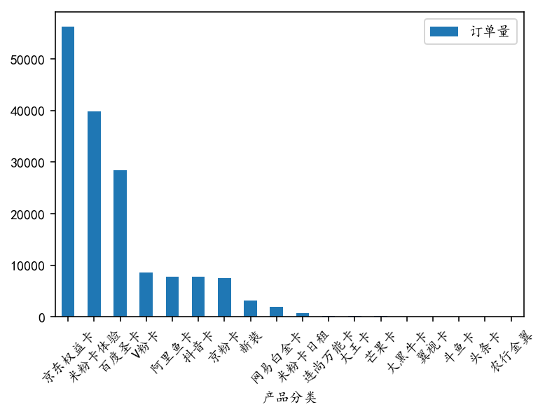
# The distribution relationship between "product classification" and "activation or non-activation" is analyzed. The graph shows that "product classification" is arranged in descending order according to "activation rate".
cp_jh_ys_c=sf_df_fahuo[['Product Classification','Activated or Not']]]. groupby(['Product Classification'], as_index=False).count()# counts orders
 cp_jh_ys_c=cp_jh_ys_c[cp_jh_ys_c['activated or not'] > 9]
cp_jh_ys_c.set_index('Product Classification', inplace=True)
cp_jh_ys_c.rename(columns = {'active or not':'order quantity'}, inplace=True)
print(cp_jh_ys_c) # View filtered data
 Product Classification Order Quantity  
V Pink Card 8583
 Jingdong Equity Card 56223
 Beijing Pink Card 7517
 Agricultural Bank Golden Wing 10
 Dawangka 242
 Daniel Niuka 99
 Head Card 10
 Jitter Card 7720
 Pisces card 19
 New 3194
 Baidu Shengka 28411
 Rice Powder Card Experience 39833
 Mifenka Daily Rent 714
 Netease Platinum Card 2012
 Wing View Card 56
 Mango Card 116
 Lianshang Universal Card 245
 Aliyuka 7737

cp_jh_ys_c.sort_values('order quantity', ascending=False).plot.bar()
pl.xticks(rotation=45)
Plt. rcParams ['figure. figsize']= (10.0, 6.0) # Sets figure_size
plt.rcParams['image.interpolation'] = 'nearest'
## The Relationship between Overall Product Classification and Activation or Not
 # cp_jh_ys=sf_df_fahuo[['Product Classification','Activated or Not']]]. groupby(['Product Classification'], as_index=False). agg (['mean','count'])  leads to a composite index that is not handled well.
cp_jh_ys_m=sf_df_fahuo[['Product Classification','Activation or Not']]]. groupby(['Product Classification'], as_index=False).mean()# Statistical Activation Rate
 cp_jh_ys_m.set_index('Product Classification', inplace=True)
cp_jh_ys_m.rename(columns = {'activated or not':'activated rate'}, inplace=True)
print(cp_jh_ys_m) # View filtered data
>>>
Product Classification Activation Rate          
V Pink Card 0.55
 Jingdong Equity Card 0.89
 Beijing Pink Card 0.69
 Agricultural Bank Golden Wing 0.60
 Dawangka 0.82
 Daniel Niuka 0.71
 Skywing Yunka 1.00
 Head Card 0.90
 Good Voice 1.00
 Vibration card 0.70
 Dogfish card 0.89
 New 0.92
 Baidu Shengka 0.54
 Rice noodle card experience 0.69
 Daily rent of rice noodle card is 0.83
 Netease Platinum Card 0.73
 Wing Visual Card 0.68
 Mango Card 0.58
 Suning Hi Card 0.75
 Lianshang Universal Card 0.65
 Aliyuka 0.67

cp_jh_ys_m.sort_values('activation rate', ascending=False).plot.bar()
Pl. xticks (rotation = 45) # Matplotlib drawing, x-axis label rotation 45 degrees
 Plt. rcParams ['figure. figsize']= (10.0, 6.0) # Sets figure_size
plt.rcParams['image.interpolation'] = 'nearest'

Conclusion:
1. According to the distribution of "order quantity" of different cards, the cards of Top6 are: Jingdong Equity Card, Mifen Card Experience, Baidu Shengka, V-Pink Card, Ali Fish Card and Vibrating Card, with an average order quantity of more than 8,000 per month.
2. According to the distribution of "activation rate" of different cards, the activation rate of cards tends to decrease with the decrease of "order quantity". Among them, the activation rate of Jingdong Equity Card in Top6 is the highest 0.89 and that of Baidu Santa Card is the lowest 0.54.

#The relationship between overall "gender" and "activation or inactivation"
mpl.rc("figure", figsize=(5,5))   #Size settings
sf_df_fahuo[['Gender','Activation or not']].groupby(['Gender']).mean().plot.bar()   #Women's activation rate is relatively high
ax.set_title("The Distribution of Sex and Activation")

Conclusion:
Through the bar chart of "the distribution of gender and activation or not", we can see that the activation rate of women is higher than that of men, which can predict that the responsibility of female consumer groups is stronger.

#Analysis of the relationship between "trading cycle" and "activation or non-activation"
sf_df_fahuo_jy=sf_df_fahuo[sf_df_fahuo['Transaction cycle']<1000]  #Very few orders with a "trading cycle" of more than 1000 hours are filtered out

#Frequency Distribution Histogram of "Transaction Cycle"
jy_jh=sf_df_fahuo_jy[['Transaction cycle','Activation or not']].groupby('Transaction cycle',as_index=False).count()
#Histogram is similar to histogram in appearance, which is used to show continuous data distribution characteristics (histogram mainly shows discrete data distribution)
mpl.rc("figure", figsize=(30,10))   # Image Size Settings
sns.distplot(jy_jh['Transaction cycle'],bins=200,kde_kws={"color":"seagreen", "lw":5 },
             hist_kws=dict(edgecolor='k',color='Teal'))  #edgecolor Set the column boundary line. color Setting Column Colors#kde_kws is a fitting curve parameter
plt.xlabel('Transaction cycle')
plt.ylabel('Order Quantity')
plt.xlim(-10,400)#Set the x-axis distribution range
sns.set_context("talk", font_scale=2, rc={'line.linewidth':2.5})  # Use talk style, font size
plt.xticks(range(0,400,15),fontsize=20,rotation=45)  #Set the scale interval

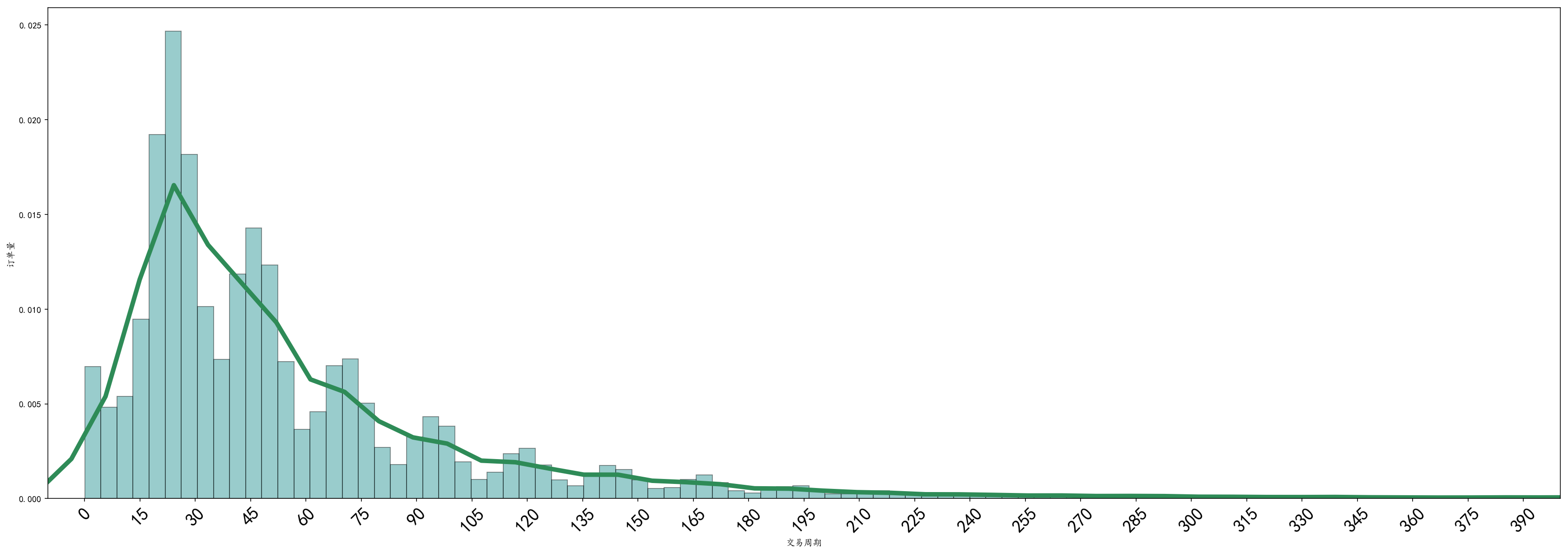
Conclusion:
1. Through the frequency distribution histogram of the "transaction cycle", we can see that the distribution of user orders approximately presents a "normal distribution" with the growth of the transaction cycle, and its right skew is more obvious, which can be optimized by "logarithmic transformation".
2. Trading cycle time-consuming is generally concentrated in the [0,96] interval, that is, within 1-4 days to complete the whole process from placing orders to signing logistics orders.
3. Observing the frequency distribution histogram of the "transaction cycle", we find that there are many intermittent peaks, with the interval difference approximating 24 hours, which is just similar to the peak distribution rule of daily logistics distribution. Moreover, combined with the time difference between the peak value and the order time, it can be inferred that users generally place orders between 8 and 12 p.m., which is also in line with the current consumer life and rest.

f,ax=plt.subplots(2,2,figsize=(30,24))  #Set the size and number of maps
sns.countplot('Gender',data=sf_df_fahuo,ax=ax[0,0],hue='Activation or not')  #Drawing gender statistics
sns.countplot('Age classification',data=sf_df_fahuo,ax=ax[0,1],hue='Activation or not')  #Draw a Statistical Map of "Age Level"
sns.countplot('Number Ownership Province',data=sf_df_fahuo,ax=ax[1,0],hue="Activation or not") #Drawing the Statistical Map of "Number Ownership Province"
sns.countplot('Product Classification',data=sf_df_fahuo,ax=ax[1,1],hue='Activation or not')
ax[0,0].set_title("Relationship Distribution between Order Quantity and Sex")   #Title Settings
ax[0,1].set_title("Distribution of Order Quantity and Age Classification")
ax[1,0].set_title("Relation Distribution between Order Quantity and Number Ownership Province")
ax[1,1].set_title("Relationship Distribution between Order Quantity and Product Classification")
# ax[1,0].set_xticklabels(ax.get_xticklabels(),rotation=-45)
# ax[0,1].set_xlabel('Age classification',fontsize=12,color='r')   #Set the "name" of the X-axis label, font size, and font color
# ax[0,1].set_ylabel('Order Quantity',fontsize=12,color='r')    #Set the name, font size and font color of the Y-axis label
ax[1,0].grid(True, linestyle='-.')  #Setting grid style
for label in ax[1,0].xaxis.get_ticklabels():
	label.set_rotation(45)   #Setting the rotation direction of the font with the x-axis scale
    label.set_fontsize(12)
#     label.set_visible(False)   # The solution is to hide some points according to the actual situation. set_visible(False) is not displayed and True is displayed.
    label.set_visible(True)

ax[1,1].grid(True,linestyle='-.')  #Setting grid style
for label in ax[1,1].get_xticklabels():
    label.set_rotation(45)
    label.set_fontsize(12)
    label.set_visible(False)
for label in ax[1,1].xaxis.get_ticklabels()[::1]:     # Solutions to over-intensive x-axis labels hide some points according to the actual situation, [::2] means two display intervals.
    label.set_visible(True)   

Conclusion:
1,
2,

# Analysis of the Relation between Product Classification and Age Classification
 sf_df_fahuo.groupby(['Product Classification','Age Classification']) ['Age Classification']. count()
>>>
Product Classification Age Classification
 V Pink Card No Confuse 762
          Juvenile 2015
          Weak crown 3766
          Destiny 413
          Old age 58
          And Li 1374
          Huajia 195
 Beijing East Equity Card No Confusion 6496
          Juvenile 1996
          Weak crown 12444
          Destiny 7471
          Age 1306
          And Li 9164
          Flower armor 17346
 Beijing Pink Card Puzzle 621
          Juvenile 372
          Weak crown 4203
          Destiny 65
          Old age 8
          And Li 2239
          Flower armor 9
 Agricultural Bank of China Golden Wing Doubtful 3
          Juvenile 1
          Weak crown 1
          Knowing Destiny 2
          And Li 3
 Dawangka Doubtful 12
          Juvenile 31
          Weak crown 160
          Knowing Destiny 4
          Old age 2
          And Li 32
          Flower armor 1
 Big Black Niuka Doubtful 10
          Juvenile 17
          Weak crown 53
          Knowing Destiny 4
          And Li 13
          Flower armor 2
 Tianyi Yunka Rili 1
 Head Card Junior 2
         Weak crown 4
         Knowing Destiny 1
         And Li 3
 Good voice knows fate 1
 Vibrating Card No. 744
         Juvenile 1266
         Weak crown 3736
         Knowing fate 373
         Old age 22
         And Li 1477
         Flower armor 102
 Fighter Card No Confuse 1
         Juvenile 1
         Weak crown 14
         And Li 3
 New clothes no puzzle 395
         Juvenile 99
         Weak crown 1326
         Zhi Ming 122
         Old age 25
         And Li 1154
         Carapace 73
 Baidu Saint Card Puzzled 970
         Juvenile 7466
         Weak crown 16151
         Knowing Fate 277
         Old age 46
         And Li 3401
         Flower armor 100
 Mifenka Experience No Confuse 4941
          Juvenile 2889
          Weak crown 15601
          Zhiming 3803
          Old age 291
          And Li 10565
          Flower armor 1743
 Mifenka Daily Rent No doubt 74
          Juvenile 32
          Weak crown 353
          Knowing Fortune 42
          Age 3
          And Li 189
          Flower armor 21
 Netease Platinum Card
          Juvenile 447
          Weak crown 1303
          Zhi Ming 20
          Old age 2
          And Li 176
          Flower armor 8
 Wing Visual Card No. 8
          Juvenile 5
          Weak crown 26
          Knowing Destiny 3
          Old age 1
          And Li 10
          Flower armor 3
 Mango Card No Puzzle 3
          Juvenile 26
	      Weak crown 78
	      Knowing Destiny 1
	      And Li 8
 Suning Hi Ka Weak Crown 2
          And Li 2
 Lianshang Universal Card
          Juvenile 12
	      Weak crown 109
	      Destiny 10
	      Old age 1
	      And Li 71
	      Flower armor 7
 Ali Fish Card No Confusion 541
	      Juvenile 586
	      Weak crown 4453
	      Knowing Destiny 255
	      Old age 22
	      And Li 1805
	      Flower armor 75
 Name: Age Classification, dtype: int64

# Distribution of "Product Classification" and "Age"
fig, ax = plt.subplots(1, 2, figsize = (30, 10))
sns.violinplot("gender", "age", "hue="activated or not"), data=sf_df_fahuo, split=True, ax=ax[0])
ax[0].set_title('sex and age vs activated or not')
ax[0].set_yticks(range(0, 110, 10))
ax[0].grid(True, linestyle='-')

sns.violinplot("Product Classification", "Age", "hue="Activated or Not"), data=sf_df_fahuo, split=True, ax=ax[1])
ax[1].set_title("Product Classification and Age vs Activated or Not")
ax[1].set_yticks(range(0,110,10))
ax[1].grid(True,linestyle='-')
for label in ax[1].get_xticklabels():
    label.set_rotation(45)
    label.set_fontsize(15)

sns.set_style('white')
f, ax = plt.subplots(figsize=(8,7))
ax = sns.boxplot(x='Age',y='Product Classification',data=sf_df_fahuo, orient='h',palette='Set1')
ax.xaxis.grid(False)
ax.set(ylabel='Classification_KP')
ax.set(xlabel='Age')
ax.set(title='Relationshape between Age and Classification_KP ')
sns.despine(trim=True,left=True)

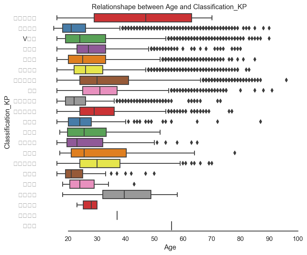
Conclusion:
1,
2,

# ax.set_title("Distribution of Product Classification and Age Classification")
cp_nj=sf_df_fahuo[['Product Classification','Age classification','Order Number']].groupby(['Product Classification','Age classification'],as_index=False).count()   #Set up#The parameter as_index=False, which converts the index column to the label of the X-axis of the "normal column" 
f,ax=plt.subplots(1,1,figsize=(30,15))  #Set the size and number of maps
sns.barplot(x='Product Classification', y='Order Number', hue="Age classification",data=cp_nj,ci=0)
plt.legend(loc = 'upper right')  #Set the legend to the top right corner
# ax.set_xlabel("va=top")  #Set the label title for the X-axis 
plt.setp(ax.get_xticklabels(), rotation=45, ha="right", rotation_mode="anchor") #Rotate the scale label and set its alignment mode

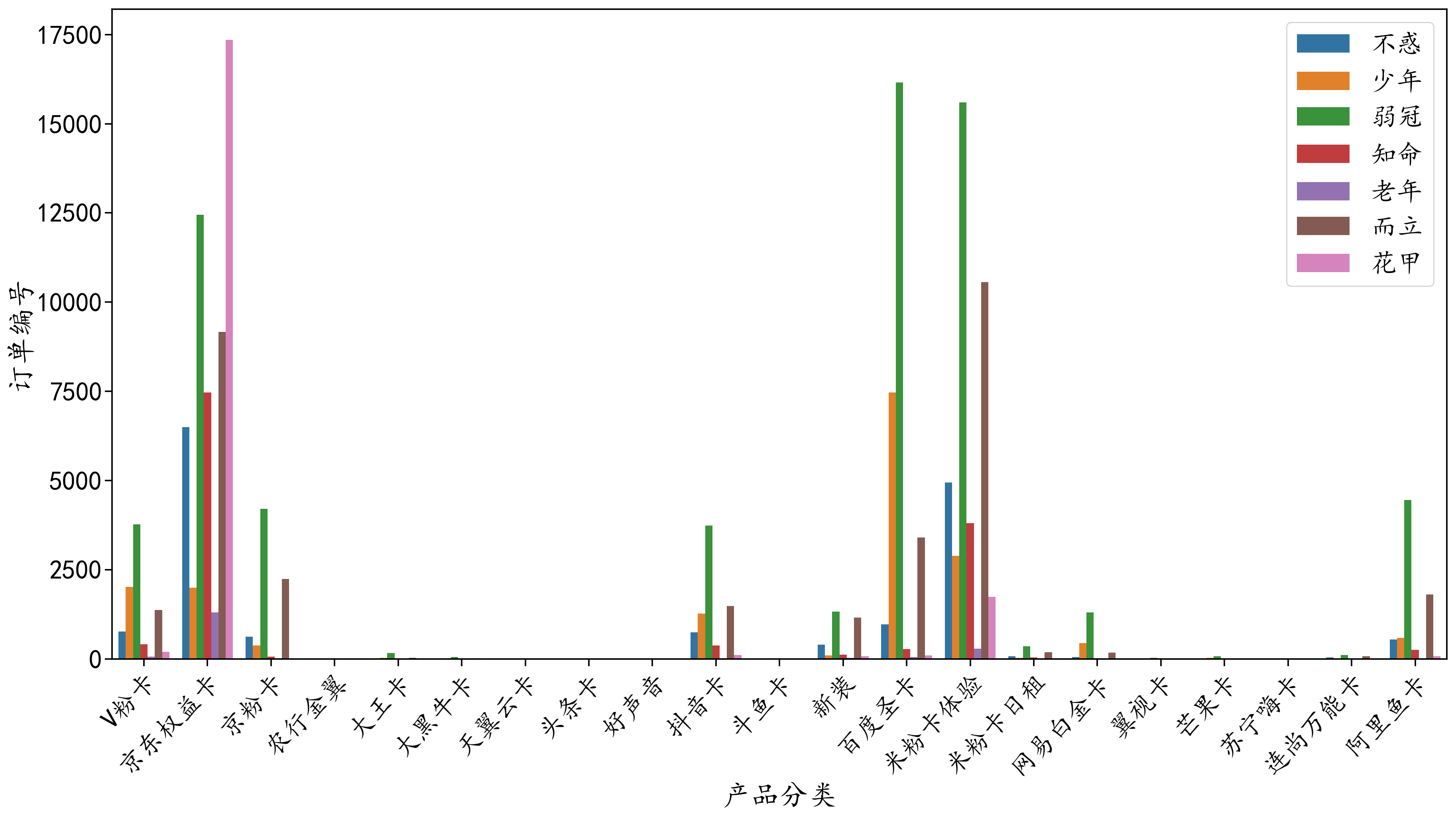
Conclusion:
1,
2,
Part02: Conversion of Characteristic Variables
The purpose of variable transformation is to transform data into data suitable for model use. Different models accept different types of data. Because Scikit-learn s require data to be digital, it is necessary to convert some non-digital raw data into digital numeric.
Qualitative transformation:
Qualitative Variables (Discrete Variables) Discrete --(1) When qualitative variables are only a few independent variables that occur frequently, Dummy Variables are more suitable for use and will increase the feature columns; (2) If the independent variables of qualitative variables have more values, factorize is used to discretize them into numeric values. The number of feature columns remains unchanged.
Binning Conversion
Continuous data are discretized by "Binning". Stored values are distributed to "buckets" or "boxes" just as bin of a histogram divides the data into blocks.

sf_df_last=sf_df_fahuo[['Order Number','Gender','Age','Age classification','Product Classification','Number Ownership Province','Transaction cycle','Activation or not']]
>>>sf_df_last.tail()
                             //Order Number, Gender, Age Classification, Product Classification, Number Belonging to Province, Transaction Cycle Activated or Not
162751	690000000001008319051324127595	male	36	While standing	   Rice noodle card experience	   Zhejiang Province	nan	    0
162752	600103832000008319051306101865	female	82	old age	   Ali Fish Card	   Jiangsu Province	80.97	1
162753	690000000001008319051324127594	female	37	While standing	   Jingdong Equity Card	   Fujian Province	0.10	1
162754	690000000001008319051324127626	female	35	While standing	   Rice noodle card experience	   Guangdong Province	27.93	1
162755	690000000001008319051324127605	male	23	Weak crown	   Rice noodle card experience	   Guangdong Province	9.65	1
print(sf_df_last['Age classification'].nunique())
print(sf_df_last['Product Classification'].nunique())  #Statistics on the number of non-repetitive items in the category of "Product Classification"
print(sf_df_last['Number Ownership Province'].nunique())
>>>
7
21
31

#The following code Binning the'trading cycle'.
sf_df_last['Transaction cycle'][sf_df_last['Transaction cycle'].isnull()]=1000  #Fill the vacancies in the "transaction cycle" column with "1000"
#Mapping the "trading cycle" to a discrete interval of one day, starting from 0.5 days, 1.5 days, 2.5 days in turn,... Until more than 9.5 days is directly classified as 10 days.
#After binning, factorize is done conveniently, that is, feature discretization.
def func_period(str1):
    if str1<=12:
        return 0.5
    elif str1<=36:
        return 1.5
    elif str1<=60:
        return 2.5
    elif str1<=84:
        return 3.5
    elif str1<=108:
        return 4.5
    elif str1<=132:
        return 5.5
    elif str1<=156:
        return 6.5
    elif str1<=180:
        return 7.5
    elif str1<=204:
        return 8.5
    elif str1<=228:
        return 9.5
    else:
        return 10
  
sf_df_last['Transaction cycle']=sf_df_last['Transaction cycle'].apply(func_period)   

#Method 1: Encoding with factoriz
sf_df_last['Gender']=pd.factorize(sf_df_last['Gender'])[0]
#Method 2: Coding with dummies
# sex_dummies_df=pd.get_dummies(sf_df_last['gender'], prefix=sf_df_last['gender']]]]. columns[0])
# sf_df_last=pd.concat([sf_df_last,sex_dummies_df],axis=1)
sf_df_last['Age classification']=pd.factorize(sf_df_last['Age classification'])[0]
sf_df_last['Number Ownership Province']=pd.factorize(sf_df_last['Number Ownership Province'])[0]
sf_df_last['Product Classification']=pd.factorize(sf_df_last['Product Classification'])[0]
sf_df_last['Transaction cycle']=pd.factorize(sf_df_last['Transaction cycle'])[0]  #Feature discretization using factorize
>>> sf_df_last.tail()  # Unithermal Coded Data Set
								//Order Number, Gender, Age Classification, Product Classification, Number Belonging to Province, Transaction Cycle Activated or Not
162751	690000000001008319051324127595	0	36	   3	   6	   24	      2	    0
162752	600103832000008319051306101865	1	82	   6	   5	   12	      5	    1
162753	690000000001008319051324127594	1	37	   3	   0	   15	      0	    1
162754	690000000001008319051324127626	1	35	   3	   6	   6	      3	    1
162755	690000000001008319051324127605	0	23	   1	   6	   6	      0    	1

Describing correlation: Generally, pairplot and heatmap graphs are used to describe correlation.

#heatmap diagram
Correlation=sf_df_last[['Gender','Age classification','Number Ownership Province','Product Classification','Transaction cycle']]

colormap = plt.cm.viridis
plt.figure(figsize=(15,15))
plt.title('Pearson Correlation of Features', y=1.05, size=20)
sns.heatmap(Correlation.astype(float).corr(),linewidths=0.1,vmax=1.0,
            square=True, cmap=colormap, linecolor='white', annot=True)
plt.xticks(rotation=45)    # Rotate fonts (X axis rotates differently in seaborn and matplotlib modes)

model training

#The training data are divided into two parts: marker and feature.
labels=sf_df_last['Activation or not']
features=sf_df_last[['Gender','Age classification','Number Ownership Province','Product Classification','Transaction cycle']]

#First, introduce the required libraries and functions
from sklearn.model_selection import GridSearchCV
from sklearn.metrics import make_scorer
from sklearn.metrics import accuracy_score,roc_auc_score
from time import time
from sklearn.tree import DecisionTreeClassifier
from sklearn.svm import SVC
from sklearn.ensemble import RandomForestClassifier
from sklearn.ensemble import AdaBoostClassifier
from sklearn.neighbors import KNeighborsClassifier
from xgboost.sklearn import XGBClassifier

#Defining a General Function Framework
def fit_model(alg,parameters):
    X=features
    y=labels #Because of the small amount of data, the whole data is used for grid search.
    scorer=make_scorer(roc_auc_score)   #Using roc_auc_score as scoring criterion
    grid=GridSearchCV(alg,parameters,scoring=scorer,cv=5)  #Using grid search, access parameters
    start=time()  #Time
    grid=grid.fit(X,y)  #model training
    end=time()
    t=round(end-start,3)
    print(grid.best_params_)  #Output optimum parameters
    print("searching time for {} is {}s".format(alg.__class__.__name__,t))  #Output search time
    return grid  #Return the trained model
#Define the initial function
#List the algorithms to be used
alg1=DecisionTreeClassifier(random_state=29)
alg2=SVC(probability=True,random_state=29)  #Since roc_auc_score is used as the scoring criterion, the probability parameter in SVC needs to be set to True.
alg3=RandomForestClassifier(random_state=29)
alg4=AdaBoostClassifier(random_state=29)
alg5=KNeighborsClassifier(n_jobs=-1)
alg6=XGBClassifier(random_state=29,n_jobs=-1)

#Listing the parameters and ranges we need to adjust is a very tedious task, which requires a lot of attempts and optimization.
parameters1={'max_depth':range(1,10),"min_samples_split":range(2,10)}
parameters2={'C':range(1,20),'gamma':[0.05,0.1,0.15,0.2,0.25]}
parameters3_1={'n_estimators':range(10,200,10)}
parameters3_2={'max_depth':range(1,10),'min_samples_split':range(2,10)} #The search space is too large to adjust the parameters twice.
parameters4={'n_estimators':range(10,200,10),'learning_rate':[i/10.0 for i in range(5,15)]}
parameters5={'n_estimators':range(2,10),'leaf_size':range(10,80,20)}
parameters6_1={'n_estimators':range(10,200,10)}
parameters6_2={'max_depth':range(1,10),'min_child_weight':range(1,10)}
parameters6_3={'subsample':[i/10.0 for i in range(1,10)],'colsample_bytree':[i/10.0 for i in range(1,10)]}  #Search space is too large to adjust parameters three times.

#Start adjusting parameters
#DecisionTreeClassifier
clf1=fit_model(alg1,parameters1)
>>>
{'max_depth': 2, 'min_samples_split': 2}
searching time for DecisionTreeClassifier is 69.031s
#SVM
clf2=fit_model(alg2,parameters2)
#RandomForest
#First adjustment of parameters
clf3_m1=fit_model(alg3,parameters3_1)
#Second adjustment of parameters
alg3=RandomForestClassifier(random_State=29,n_estimators=10)
clf3=fit_model(alg3,parameters3_2)
#AdaBoost
clf4=fit_model(alg4,parameters4)
#KNN
clf5=fit_model(alg5,parameters5)
#Xgboost
#First adjustment of parameters
clf6_m1=fit_model(alg6,parameters6_1)
#Second adjustment of parameters
alg6=XGBClassifier(n_estimators=140,random_state=29,n_jobs=-1)
clf6_m2=fit_model(alg6,parameters6_2)
#Third adjustment of parameters
alg6=XGBClassifier(n_estimators=140,max_depth=4,min_child_weight=5,random_state=29,n_jobs=-1)
clf6=fit_model(alg6,parameters6_3)

#Now that the process of parameter adjustment and training is over, we have trained six models, and now it is time to test the results.
#First, a save function is defined to save the predicted results in a submissible format.
def save(clf,i):
    pred=clf.predict(test)
    sub=pd.DataFrame({'Order Number':,'Activation or not':})
    sub.to_csv('res_tan_{}.csv'.format(i),index=False)
#Call this function to complete the prediction of six models:
i=1
for clf in [clf1,clf2,clf3,clf4,clf5,clf6]:
    save(clf,i)
    i=i+1