Then we look at the more complex application of LSTM network, which is used to predict temperature. In this example, we can use many advanced data processing functions. For example, we can see how to use "recurrent dropout" to prevent overfitting. Second, we will stack multiple LTSM network layers to enhance the resolution ability of each network. Third, we will also use two-way recurrent networks, It will transfer the same information in different forms in the network, so as to increase the network's understanding of information.

The first important step we need to do is to obtain the data, open Xunlei and enter the following URL to download the original data: https://s3.amazonaws.com/keras-datasets/jena_climate_2009_2016.csv.zip After downloading and decompressing, we can load it into memory with code:

import os
data_dir = '/Users/chenyi/Documents/artificial intelligence/'
fname = os.path.join(data_dir, 'jena_climate_2009_2016.csv')f = open(fname)
data = f.read()
f.close()lines = data.split('\n')
header = lines[0].split(',')
lines = lines[1:]print(header)
print(len(lines))

After running the above code, the results are as follows: ['"Date Time"', '"p (mbar)"', '"T (degC)"', '"Tpot (K)"', '"Tdew (degC)"', '"rh (%)"', '"VPmax (mbar)"', '"VPact (mbar)"', '"VPdef (mbar)"', '"sh (g/kg)"', '"H2OC (mmol/mol)"', '"rho (g/m**3)"', '"wv (m/s)"', '"max. wv (m/s)"', '"wd (deg)"'] 420551 There are 420551 entries in total, and the content of each entry is shown above. Next, we convert all entries into an array format that can be processed:

import numpy as np
float_data = np.zeros((len(lines), len(header) - 1))
for i, line in enumerate(lines):
   values = [float(x) for x in line.split(',')[1:]]
   float_data[i, :] = valuesfrom matplotlib import pyplot as plt
temp = float_data[:, 1]
plt.plot(range(len(temp)), temp)

After the above transcoding data, the data is depicted, and the results are as follows:

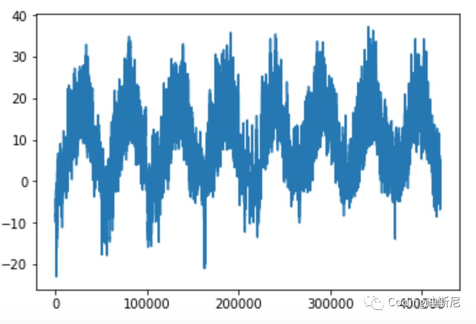
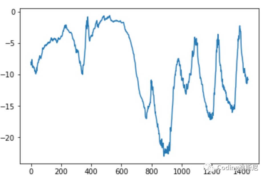
As can be seen from the above figure, the temperature presents a periodic change. Since the data records the daily temperature changes from 2009 to 2016, and the temperature records are completed every ten minutes, there are 144 recording points a day. We intercept the temperature information for 10 days, that is, a total of 1440 data points. Let's draw these data graphs:

plt.plot(range(1440), temp[:1440])

We will construct a network, analyze the current weather data, and then predict the possible weather conditions in the future. The current data format is ideal. The problem is that the units corresponding to different data are different. For example, air temperature and air pressure adopt different measurement units. Therefore, we need to normalize the data. We intend to use the first 200000 data items as training data, so we only normalize this part of data:

mean = float_data[:200000].mean(axis=0)
float_data -= mean
std = float_data[:200000].std(axis=0)
float_data /= std

Then we use code to divide the data into three groups. One group is used to train the network, one group is used as verification data, and the last group is used as test data:

'''
Suppose it is 1 o'clock now, we want to predict the temperature at 2 o'clock, because the current data records the meteorological data every 10 minutes, from 1 o'clock to 2 o'clock
 The interval is 1 hour, corresponding to 6 10 minutes. This 6 corresponds to delay To train the network to predict temperature, we need to establish a corresponding relationship between meteorological data and temperature. We can push back 10 days from 1 o'clock, starting from the past
10 The training data is formed after sampling in the meteorological data of days. Since the meteorological data is recorded every 10 minutes, the backward 10 days is from
 At the current time, 1440 pieces of data are traced back. This 1440 corresponds to lookback Instead of taking all 1440 data as training data, we sample from these data and take one every 6,
So there are 1440/6=240 This data will be used as training data, which is the training data in the code lookback//step so I took the sampling data within 10 days before 1 o'clock as the training data, and the temperature at 2 o'clock as the correct answer corresponding to the data
 The network can be trained
'''
def generator(data, lookback, delay, min_index, max_index, shuffle=False,
            batch_size=128, step=6):
   if max_index is None:
       max_index = len(data) - delay - 1
   i = min_index + lookback
   while 1:
       if shuffle:
           rows = np.random.randint(min_index + lookback, max_index, size=batch_size)
       else:
           if i + batch_size >= max_index:
               i = min_index + lookback
           rows = np.arange(i, min(i + batch_size, max_index))
           i += len(rows)
       samples = np.zeros((len(rows), lookback//step, data.shape[-1]))
       targets = np.zeros((len(rows), ))
       for j, row in enumerate(rows):
           indices = range(rows[j] - lookback, rows[j], step)
           samples[j] = data[indices]
           targets[j] = data[rows[j] + delay][1]
       yield samples, targets

With the above data processing function, we can call it to divide the original data into three groups, one for training, one for verification and the last for testing. The code is as follows:

lookback = 1440
step = 6
delay = 144
batch_size = 128train_gen = generator(float_data, lookback=lookback,
                     delay=delay, min_index=0,
                     max_index=200000, shuffle=True,
                     step=step,batch_size=batch_size)
val_gen = generator(float_data, lookback=lookback,
                  delay=delay, min_index=200001,
                  max_index=300000,
                  step=step, batch_size=batch_size)
test_gen = generator(float_data, lookback=lookback,
                  delay=delay, min_index=300001,
                  max_index=400000,
                  step=step, batch_size=batch_size)val_steps = (300000 - 200001 - lookback) // batch_size
test_steps = (len(float_data) - 300001 - lookback) //batch_size

To be effective, neural network must do better than human prediction. For temperature prediction, people instinctively think that the temperature is continuous, that is, the temperature at the next moment should not be much different from that at the current moment. According to people's experience, it is impossible that the current temperature is 20 degrees, and then the temperature at the next moment becomes 60 degrees, or minus 20 degrees. Only the end of the world will happen. Therefore, if people want to predict, He usually thinks that the temperature in the next 24 hours is the same as the current temperature. Based on this logic, we calculate the accuracy of this prediction method:

def  evaluate_naive_method():
   batch_maes = []
   for step in range(val_steps):
       samples, targets = next(val_gen)
       #preds is the temperature at the current time and targets is the temperature in the next hour
       preds = samples[:, -1, 1]
       mae = np.mean(np.abs(preds - targets))
       batch_maes.append(mae)
   print(np.mean(batch_maes))
evaluate_naive_method()

After running the above code, the result is 0.29. Note that we have normalized each column of data, so the interpretation of 0.29 should be 0.29*std[1]=2.57, that is, if we use the temperature of the previous hour to predict the temperature of the next hour, the error is 2.57 degrees, which is not small. If our network is really effective, its predicted temperature error should be smaller than 2.57. The smaller it is, the more effective it is.

In order to compare the effects of different network models, we will construct several different types of networks, and then look at their prediction effects. First, we will establish the fully connected network described in the previous chapters to see the effect:

from keras.models import Sequential
from keras import layers
from keras.optimizers import RMSpropmodel = Sequential()
model.add(layers.Flatten(input_shape=(lookback // step,
                                     float_data.shape[-1])))
model.add(layers.Dense(32, activation='relu'))
model.add(layers.Dense(1))model.compile(optimizer=RMSprop(), loss='mae')
history = model.fit_generator(train_gen, steps_per_epoch=500,
                            epochs=20,
                            validation_data=val_gen,
                            validation_steps=val_steps)

Let's draw the running results of the above code:

import matplotlib.pyplot as plt
loss = history.history['loss']
val_loss = history.history['val_loss']
epochs = range(1, len(loss) + 1)
plt.figure()plt.plot(epochs, loss, 'bo', label='Training loss')
plt.plot(epochs, val_loss, 'b', label='Validation loss')
plt.title('Training and Validation loss')plt.show()

After running the above code, the results are as follows:

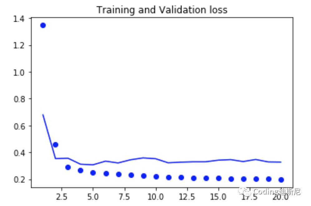
From the above figure, the result of network prediction is between 0.4 and 0.3, which means that the accuracy of network prediction is not as good as people's intuition. There is a problem in the current network, that is, it flattens the data items with time order at once, so that the time relationship between the data disappears. However, the time information is very important for the prediction of the results. If multiple data are collected together and transmitted to the network like the above method, the time characteristics of the data will disappear, Time is an important variable affecting the judgment results.

This time we use the recurrent neural network, because such a network can use the time relationship between data to analyze the potential laws of data, so as to improve the accuracy of prediction. The recurrent network we use this time is called GRU, which is a variant of LSTM. The basic principles of the two are the same, but the former is the optimization of the latter, so that the efficiency can be accelerated during training, Let's look at the relevant codes:

model = Sequential()
model.add(layers.GRU(32, input_shape=(None, float_data.shape[-1])))
model.add(layers.Dense(1))model.compile(optimizer=RMSprop(), loss='mae')
history = model.fit_generator(train_gen, steps_per_epoch=500,
                      epochs = 20, validation_data=val_gen,
                      validation_steps=val_steps)

After the code is run, the training effect we draw is as follows:

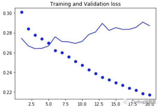
We can see from the above figure that when the number of cycles of the blue solid line is 4, the error of the network in judging the verification data is close to 0.26, which is far better than the 0.29 error rate guessed by human intuition. This improvement is quite obvious. This improvement shows that the ability of deep learning to extract data patterns is much better than human intuition. At the same time, it also shows that the recognition ability of recurrent network is better than the fully connected network we developed before. The error value converted from 0.26 is about 2.3, that is, the temperature predicted by the network after one hour is 2.3 degrees different from the actual value.

From the above figure, we can also see that the recognition accuracy of the network for training data is increasing, and the recognition accuracy of the verification data is getting worse and worse. The two parted ways are obvious, that is to say, there is over fitting in the network. In the past, we used to reset the weights randomly when dealing with over fitting, but this method can not be directly used in the repetitive network, because many link weights in the network are used to record the internal correlation of different data in time. If these weights are reset randomly, the network's understanding of the temporal correlation of data will be destroyed, resulting in the decline of accuracy. In 2015, Yarin Gal, a doctoral student who studied Bayesian deep learning, found a method to deal with the over fitting of recurrent networks. That is to clear the same proportional weights every time, rather than randomly, and this clearing mechanism is embedded in the keras framework. Relevant codes are as follows:

model = Sequential()
model.add(layers.GRU(32, dropout=0.2, recurrent_dropout=0.2,
                   input_shape=(None, float_data.shape[-1])))
model.add(Dense(1))
model.compile(optimizer=RMSprop(), loss='mae')
history = model.fit_generator(train_gen, steps_per_epoch=500,
                            epochs = 40, validation_data=val_gen,
                            validation_steps = val_steps)

After the above code is run, the training effect of the network is as follows:

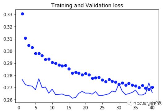
From the above figure, the development trend of point and line continues to coincide, that is, the recognition accuracy of verification data by the network continues to improve as the accuracy of training data, so the phenomenon of over fitting disappears. So far, we have demonstrated the application of LSTM and GRU in specific examples. If you have run the above code, you will find that the code running efficiency of ordinary CPU is very slow. It proves once again that computing power and data are two very difficult difficulties in artificial intelligence.