definition
In addition to retrieval, ES also provides statistical analysis of data, with high real-time performance
Bucket aggregation
Filter out documents that meet specific criteria:
GET kibana_sample_data_flights/_search
{
  "size": 0,
  "aggs": {
    "dest": {
      "terms": {
        "field": "DestCountry"
      }
    }
  }
}
The output is as follows. You can see the number of flights to each country in the aggregation:
{
  "took" : 4,
  "timed_out" : false,
  "_shards" : {
    "total" : 1,
    "successful" : 1,
    "skipped" : 0,
    "failed" : 0
  },
  "hits" : {
    "total" : {
      "value" : 10000,
      "relation" : "gte"
    },
    "max_score" : null,
    "hits" : [ ]
  },
  "aggregations" : {
    "dest" : {
      "doc_count_error_upper_bound" : 0,
      "sum_other_doc_count" : 3187,
      "buckets" : [
        {
          "key" : "IT",
          "doc_count" : 2371
        },
        {
          "key" : "US",
          "doc_count" : 1987
        },
        {
          "key" : "CN",
          "doc_count" : 1096
        },
        {
          "key" : "CA",
          "doc_count" : 944
        },
        {
          "key" : "JP",
          "doc_count" : 774
        },
        {
          "key" : "RU",
          "doc_count" : 739
        },
        {
          "key" : "CH",
          "doc_count" : 691
        },
        {
          "key" : "GB",
          "doc_count" : 449
        },
        {
          "key" : "AU",
          "doc_count" : 416
        },
        {
          "key" : "PL",
          "doc_count" : 405
        }
      ]
    }
  }
}
Metric aggregation
Some mathematical operations are provided to perform statistical analysis on document fields
GET kibana_sample_data_flights/_search
{
  "size": 0,
  "aggs": {
    "dest": {
      "terms": {
        "field": "DestCountry"
      },
      "aggs": {
        "avg_price": {
          "avg": {
            "field":   "AvgTicketPrice"
          }
        },
        "max_price": {
          "max": {
            "field": "AvgTicketPrice"
          }
        },
        "min_price": {
          "min": {
            "field": "AvgTicketPrice"
          }
        }
      }
    }
  }
}
The output is as follows. You can see the average, maximum and minimum fares of flights to various countries:
{
  "took" : 1,
  "timed_out" : false,
  "_shards" : {
    "total" : 1,
    "successful" : 1,
    "skipped" : 0,
    "failed" : 0
  },
  "hits" : {
    "total" : {
      "value" : 10000,
      "relation" : "gte"
    },
    "max_score" : null,
    "hits" : [ ]
  },
  "aggregations" : {
    "dest" : {
      "doc_count_error_upper_bound" : 0,
      "sum_other_doc_count" : 3187,
      "buckets" : [
        {
          "key" : "IT",
          "doc_count" : 2371,
          "max_price" : {
            "value" : 1195.3363037109375
          },
          "min_price" : {
            "value" : 100.57646942138672
          },
          "avg_price" : {
            "value" : 586.9627099618385
          }
        },
        {
          "key" : "US",
          "doc_count" : 1987,
          "max_price" : {
            "value" : 1199.72900390625
          },
          "min_price" : {
            "value" : 100.14596557617188
          },
          "avg_price" : {
            "value" : 595.7743908825026
          }
        },
        {
          "key" : "CN",
          "doc_count" : 1096,
          "max_price" : {
            "value" : 1198.4901123046875
          },
          "min_price" : {
            "value" : 102.90382385253906
          },
          "avg_price" : {
            "value" : 640.7101617033464
          }
        },
        {
          "key" : "CA",
          "doc_count" : 944,
          "max_price" : {
            "value" : 1198.8525390625
          },
          "min_price" : {
            "value" : 100.5572509765625
          },
          "avg_price" : {
            "value" : 648.7471090413757
          }
        },
        {
          "key" : "JP",
          "doc_count" : 774,
          "max_price" : {
            "value" : 1199.4913330078125
          },
          "min_price" : {
            "value" : 103.97209930419922
          },
          "avg_price" : {
            "value" : 650.9203447346847
          }
        },
        {
          "key" : "RU",
          "doc_count" : 739,
          "max_price" : {
            "value" : 1196.7423095703125
          },
          "min_price" : {
            "value" : 101.0040054321289
          },
          "avg_price" : {
            "value" : 662.9949632162009
          }
        },
        {
          "key" : "CH",
          "doc_count" : 691,
          "max_price" : {
            "value" : 1196.496826171875
          },
          "min_price" : {
            "value" : 101.3473129272461
          },
          "avg_price" : {
            "value" : 575.1067587028537
          }
        },
        {
          "key" : "GB",
          "doc_count" : 449,
          "max_price" : {
            "value" : 1197.78564453125
          },
          "min_price" : {
            "value" : 111.34574890136719
          },
          "avg_price" : {
            "value" : 650.5326856005696
          }
        },
        {
          "key" : "AU",
          "doc_count" : 416,
          "max_price" : {
            "value" : 1197.6326904296875
          },
          "min_price" : {
            "value" : 102.2943115234375
          },
          "avg_price" : {
            "value" : 669.5588319668403
          }
        },
        {
          "key" : "PL",
          "doc_count" : 405,
          "max_price" : {
            "value" : 1185.43701171875
          },
          "min_price" : {
            "value" : 104.28328704833984
          },
          "avg_price" : {
            "value" : 662.4497233072917
          }
        }
      ]
    }
  }
}
Pipeline aggregation
Conduct secondary polymerization on other polymerization results.
The above statistical fare is an example of aggregation. Here is an example of statistical weather:
GET kibana_sample_data_flights/_search
{
  "size": 0,
  "aggs": {
    "dest": {
      "terms": {
        "field": "DestCountry"
      },

      "aggs": {
        "weather": {
          "terms": {
            "field": "DestWeather"
          }
        }
      }
    }
  }
}
The results are as follows:
{
"took" : 18,
"timed_out" : false,
"_shards" : {
"total" : 1,
"successful" : 1,
"skipped" : 0,
"failed" : 0
},
"hits" : {
"total" : {
"value" : 10000,
"relation" : "gte"
},
"max_score" : null,
"hits" : [ ]
},
"aggregations" : {
"dest" : {
"doc_count_error_upper_bound" : 0,
"sum_other_doc_count" : 3187,
"buckets" : [
{
"key" : "IT",
"doc_count" : 2371,
"weather" : {
"doc_count_error_upper_bound" : 0,
"sum_other_doc_count" : 0,
"buckets" : [
{
"key" : "Clear",
"doc_count" : 428
},
{
"key" : "Sunny",
"doc_count" : 424
},
{
"key" : "Rain",
"doc_count" : 417
},
{
"key" : "Cloudy",
"doc_count" : 414
},
{
"key" : "Heavy Fog",
"doc_count" : 182
},
{
"key" : "Damaging Wind",
"doc_count" : 173
},
{
"key" : "Hail",
"doc_count" : 169
},
{
"key" : "Thunder & Lightning",
"doc_count" : 164
}
]
}
},
{
"key" : "US",
"doc_count" : 1987,
"weather" : {
"doc_count_error_upper_bound" : 0,
"sum_other_doc_count" : 0,
"buckets" : [
{
"key" : "Rain",
"doc_count" : 371
},
{
"key" : "Clear",
"doc_count" : 346
},
{
"key" : "Sunny",
"doc_count" : 345
},
{
"key" : "Cloudy",
"doc_count" : 330
},
{
"key" : "Heavy Fog",
"doc_count" : 157
},
{
"key" : "Thunder & Lightning",
"doc_count" : 155
},
{
"key" : "Hail",
"doc_count" : 142
},
{
"key" : "Damaging Wind",
"doc_count" : 141
}
]
}
},
{
"key" : "CN",
"doc_count" : 1096,
"weather" : {
"doc_count_error_upper_bound" : 0,
"sum_other_doc_count" : 0,
"buckets" : [
{
"key" : "Sunny",
"doc_count" : 209
},
{
"key" : "Rain",
"doc_count" : 207
},
{
"key" : "Clear",
"doc_count" : 192
},
{
"key" : "Cloudy",
"doc_count" : 173
},
{
"key" : "Thunder & Lightning",
"doc_count" : 86
},
{
"key" : "Hail",
"doc_count" : 81
},
{
"key" : "Heavy Fog",
"doc_count" : 79
},
{
"key" : "Damaging Wind",
"doc_count" : 69
}
]
}
},
{
"key" : "CA",
"doc_count" : 944,
"weather" : {
"doc_count_error_upper_bound" : 0,
"sum_other_doc_count" : 0,
"buckets" : [
{
"key" : "Clear",
"doc_count" : 197
},
{
"key" : "Rain",
"doc_count" : 173
},
{
"key" : "Cloudy",
"doc_count" : 156
},
{
"key" : "Sunny",
"doc_count" : 148
},
{
"key" : "Damaging Wind",
"doc_count" : 80
},
{
"key" : "Thunder & Lightning",
"doc_count" : 69
},
{
"key" : "Heavy Fog",
"doc_count" : 62
},
{
"key" : "Hail",
"doc_count" : 59
}
]
}
},
{
"key" : "JP",
"doc_count" : 774,
"weather" : {
"doc_count_error_upper_bound" : 0,
"sum_other_doc_count" : 0,
"buckets" : [
{
"key" : "Rain",
"doc_count" : 152
},
{
"key" : "Sunny",
"doc_count" : 138
},
{
"key" : "Clear",
"doc_count" : 130
},
{
"key" : "Cloudy",
"doc_count" : 123
},
{
"key" : "Damaging Wind",
"doc_count" : 66
},
{
"key" : "Heavy Fog",
"doc_count" : 58
},
{
"key" : "Thunder & Lightning",
"doc_count" : 57
},
{
"key" : "Hail",
"doc_count" : 50
}
]
}
},
{
"key" : "RU",
"doc_count" : 739,
"weather" : {
"doc_count_error_upper_bound" : 0,
"sum_other_doc_count" : 0,
"buckets" : [
{
"key" : "Cloudy",
"doc_count" : 149
},
{
"key" : "Rain",
"doc_count" : 128
},
{
"key" : "Clear",
"doc_count" : 122
},
{
"key" : "Sunny",
"doc_count" : 117
},
{
"key" : "Thunder & Lightning",
"doc_count" : 62
},
{
"key" : "Hail",
"doc_count" : 56
},
{
"key" : "Damaging Wind",
"doc_count" : 55
},
{
"key" : "Heavy Fog",
"doc_count" : 50
}
]
}
},
{
"key" : "CH",
"doc_count" : 691,
"weather" : {
"doc_count_error_upper_bound" : 0,
"sum_other_doc_count" : 0,
"buckets" : [
{
"key" : "Cloudy",
"doc_count" : 135
},
{
"key" : "Sunny",
"doc_count" : 134
},
{
"key" : "Clear",
"doc_count" : 128
},
{
"key" : "Rain",
"doc_count" : 115
},
{
"key" : "Heavy Fog",
"doc_count" : 51
},
{
"key" : "Hail",
"doc_count" : 46
},
{
"key" : "Damaging Wind",
"doc_count" : 41
},
{
"key" : "Thunder & Lightning",
"doc_count" : 41
}
]
}
},
{
"key" : "GB",
"doc_count" : 449,
"weather" : {
"doc_count_error_upper_bound" : 0,
"sum_other_doc_count" : 0,
"buckets" : [
{
"key" : "Rain",
"doc_count" : 93
},
{
"key" : "Sunny",
"doc_count" : 81
},
{
"key" : "Clear",
"doc_count" : 77
},
{
"key" : "Cloudy",
"doc_count" : 71
},
{
"key" : "Heavy Fog",
"doc_count" : 34
},
{
"key" : "Hail",
"doc_count" : 32
},
{
"key" : "Damaging Wind",
"doc_count" : 31
},
{
"key" : "Thunder & Lightning",
"doc_count" : 30
}
]
}
},
{
"key" : "AU",
"doc_count" : 416,
"weather" : {
"doc_count_error_upper_bound" : 0,
"sum_other_doc_count" : 0,
"buckets" : [
{
"key" : "Rain",
"doc_count" : 80
},
{
"key" : "Cloudy",
"doc_count" : 75
},
{
"key" : "Clear",
"doc_count" : 73
},
{
"key" : "Sunny",
"doc_count" : 57
},
{
"key" : "Hail",
"doc_count" : 38
},
{
"key" : "Thunder & Lightning",
"doc_count" : 34
},
{
"key" : "Heavy Fog",
"doc_count" : 32
},
{
"key" : "Damaging Wind",
"doc_count" : 27
}
]
}
},
{
"key" : "PL",
"doc_count" : 405,
"weather" : {
"doc_count_error_upper_bound" : 0,
"sum_other_doc_count" : 0,
"buckets" : [
{
"key" : "Clear",
"doc_count" : 74
},
{
"key" : "Rain",
"doc_count" : 71
},
{
"key" : "Cloudy",
"doc_count" : 67
},
{
"key" : "Sunny",
"doc_count" : 66
},
{
"key" : "Thunder & Lightning",
"doc_count" : 37
},
{
"key" : "Damaging Wind",
"doc_count" : 30
},
{
"key" : "Hail",
"doc_count" : 30
},
{
"key" : "Heavy Fog",
"doc_count" : 30
}
]
}
}
]
}
}
}
Let's take another look at using buckets_path specifies an example of the hierarchical relationship of the aggregation, where min_bucket is the minimum value:
POST employees/_search
{
  "size": 0,
  "aggs": {
    "jobs": {
      "terms": {
        "field": "job.keyword",
        "size": 10
      },
      "aggs": {
        "avg_salary": {
          "avg": {
            "field": "salary"
          }
        }
      }
    },
    "min_salary_by_job": {
      "min_bucket": {
        "buckets_path": "jobs>avg_salary"
      }
    }
  }
}
The above effect is to find the type of work with the lowest average wage, and the final output is the result
    "min_salary_by_job" : {
      "value" : 19250.0,
      "keys" : [
        "Javascript Programmer"
      ]
    }
Replace min above with max to find the highest; Changing min into avg is to find the average of the bucket; Instead, stats is to output information such as maximum, minimum and average.
Matrix aggregation
Operate on multiple fields and provide a result matrix
Scope of polymerization
The default range is the query result set of query. It also supports changing the scope of aggregation in the following ways: Filter, PostFieldr and Global.
First change the Mapping of the employees index:
DELETE /employees

PUT /employees/
{
  "mappings": {
    "properties": {
      "age": {
        "type": "integer"
      },
      "gender": {
        "type": "keyword"
      },
      "job": {
        "type": "text",
        "fields": {
          "keyword": {
            "type": "keyword",
            "ignore_above": 50
          }
        }
      },
      "name": {
        "type": "keyword"
      },
      "salary": {
        "type": "integer"
      }
    }
  }
}
Then insert the data:
PUT /employees/_bulk
{ "index" : {  "_id" : "1" } }
{ "name" : "Emma","age":32,"job":"Product Manager","gender":"female","salary":35000 }
{ "index" : {  "_id" : "2" } }
{ "name" : "Underwood","age":41,"job":"Dev Manager","gender":"male","salary": 50000}
{ "index" : {  "_id" : "3" } }
{ "name" : "Tran","age":25,"job":"Web Designer","gender":"male","salary":18000 }
{ "index" : {  "_id" : "4" } }
{ "name" : "Rivera","age":26,"job":"Web Designer","gender":"female","salary": 22000}
{ "index" : {  "_id" : "5" } }
{ "name" : "Rose","age":25,"job":"QA","gender":"female","salary":18000 }
{ "index" : {  "_id" : "6" } }
{ "name" : "Lucy","age":31,"job":"QA","gender":"female","salary": 25000}
{ "index" : {  "_id" : "7" } }
{ "name" : "Byrd","age":27,"job":"QA","gender":"male","salary":20000 }
{ "index" : {  "_id" : "8" } }
{ "name" : "Foster","age":27,"job":"Java Programmer","gender":"male","salary": 20000}
{ "index" : {  "_id" : "9" } }
{ "name" : "Gregory","age":32,"job":"Java Programmer","gender":"male","salary":22000 }
{ "index" : {  "_id" : "10" } }
{ "name" : "Bryant","age":20,"job":"Java Programmer","gender":"male","salary": 9000}
{ "index" : {  "_id" : "11" } }
{ "name" : "Jenny","age":36,"job":"Java Programmer","gender":"female","salary":38000 }
{ "index" : {  "_id" : "12" } }
{ "name" : "Mcdonald","age":31,"job":"Java Programmer","gender":"male","salary": 32000}
{ "index" : {  "_id" : "13" } }
{ "name" : "Jonthna","age":30,"job":"Java Programmer","gender":"female","salary":30000 }
{ "index" : {  "_id" : "14" } }
{ "name" : "Marshall","age":32,"job":"Javascript Programmer","gender":"male","salary": 25000}
{ "index" : {  "_id" : "15" } }
{ "name" : "King","age":33,"job":"Java Programmer","gender":"male","salary":28000 }
{ "index" : {  "_id" : "16" } }
{ "name" : "Mccarthy","age":21,"job":"Javascript Programmer","gender":"male","salary": 16000}
{ "index" : {  "_id" : "17" } }
{ "name" : "Goodwin","age":25,"job":"Javascript Programmer","gender":"male","salary": 16000}
{ "index" : {  "_id" : "18" } }
{ "name" : "Catherine","age":29,"job":"Javascript Programmer","gender":"female","salary": 20000}
{ "index" : {  "_id" : "19" } }
{ "name" : "Boone","age":30,"job":"DBA","gender":"male","salary": 30000}
{ "index" : {  "_id" : "20" } }
{ "name" : "Kathy","age":29,"job":"DBA","gender":"female","salary": 20000}
Scope: query result set
An example of using the query result set as the scope by default is as follows
POST employees/_search
{
  "size": 0,
  "query": {
    "range": {
      "age": {
        "gte": 30
      }
    }
  },
  "aggs": {
    "jobs": {
      "terms": {
        "field": "job.keyword"
      }
    }
  }
}
The output will see the information of each bucket
{
  ....
  "hits" : {
    "total" : {
      "value" : 10,
      "relation" : "eq"
    },
    ...
  },
  "aggregations" : {
    "jobs" : {
      ...
      "buckets" : [
        {
          "key" : "Java Programmer",
          "doc_count" : 5
        },
        {
          "key" : "DBA",
          "doc_count" : 1
        },
        ....
      ]
    }
  }
}
Change the scope of action through filter
An example of using filter to change the scope of action of aggs is as follows:
POST employees/_search
{
  "size": 0,
  "aggs": {
    "older_person": {
      "filter": {
        "range": {
          "age": {
            "from": 35
          }
        }
      },
      "aggs": {
        "jobs": {
          "terms": {
            "field": "job.keyword"
          }
        }
      }
    },
    "all_jobs": {
        "terms": {
          "field": "job.keyword"
        }
      }
  }
}
The filter inside will only let the elder_ The aggregation of person only works in the data with age ≥ 35, the following all_jobs is a control group. older_ The output of person is as follows
"older_person" : {
      "doc_count" : 2,
      "jobs" : {
        "doc_count_error_upper_bound" : 0,
        "sum_other_doc_count" : 0,
        "buckets" : [
          {
            "key" : "Dev Manager",
            "doc_count" : 1
          },
          {
            "key" : "Java Programmer",
            "doc_count" : 1
          }
        ]
      }
Via post_filter changes the scope of action
Using post_ An example of changing the aggregation scope of filter is as follows. Its function is to filter out qualified data in aggregation
POST employees/_search
{
  "aggs": {
    "jobs": {
      "terms": {
        "field": "job.keyword"
      }
    }
  },
  "post_filter": {
    "match": {
      "job.keyword": "Dev Manager"
    }
  }
}
The output is as follows. Dev Manager will be selected from the aggregation results
{
 ....
  "hits" : {
    ...
    "hits" : [
      {
        "_index" : "employees",
        "_type" : "_doc",
        "_id" : "2",
        "_score" : 1.0,
        "_source" : {
          "name" : "Underwood",
          "age" : 41,
          "job" : "Dev Manager",
          "gender" : "male",
          "salary" : 50000
        }
      }
    ]
  },
  "aggregations" : {
    "jobs" : {
      ...
      "buckets" : [
        {
          "key" : "Java Programmer",
          "doc_count" : 7
        },
        {
          "key" : "Javascript Programmer",
          "doc_count" : 4
        },
        ....
        {
          "key" : "Dev Manager",
          "doc_count" : 1
        },
        ...
      ]
    }
  }
}
Global global aggregation
An example of global aggregation using global is as follows, which ignores the conditions defined by query
POST employees/_search
{
  "size": 0,
  "query": {
    "range": {
      "age": {
        "gte": 40
      }
    }
  },
  "aggs": {
    "jobs": {
      "terms": {
        "field": "job.keyword"
      }
    },
    "all": {
      "global": {},
      "aggs": {
        "avg_salary": {
          "avg": {
            "field": "salary"
          }
        }
      }
    }
  }
}
The output is as follows. It can be seen that jobs aggregation will output the job types of employees ≥ 40 years old, while all will output the average salary of all
  "aggregations" : {
    "all" : {
      "doc_count" : 20,
      "avg_salary" : {
        "value" : 24700.0
      }
    },
    "jobs" : {
      ...
      "buckets" : [
        {
          "key" : "Dev Manager",
          "doc_count" : 1
        }
      ]
    }
  }
sort
Aggregate sorting, sorting by specifying order. The following example queries documents with age ≥ 20, and sorts the aggregation results in ascending order of document number and then descending order of work type
POST employees/_search
{
  "size": 0,
  "query": {
    "range": {
      "age": {
        "gte": 20
      }
    }
  },
  "aggs": {
    "jobs": {
      "terms": {
        "field": "job.keyword",
        "order": [
          {"_count": "asc"},
          {"_key": "desc"}
          ]
      }
    }
  }
}
The output results are as follows
  "aggregations" : {
    "jobs" : {
      ...
      "buckets" : [
        {
          "key" : "Product Manager",
          "doc_count" : 1
        },
        {
          "key" : "Dev Manager",
          "doc_count" : 1
        },
        {
          "key" : "Web Designer",
          "doc_count" : 2
        },
        {
          "key" : "DBA",
          "doc_count" : 2
        },
        {
          "key" : "QA",
          "doc_count" : 3
        },
        {
          "key" : "Javascript Programmer",
          "doc_count" : 4
        },
        {
          "key" : "Java Programmer",
          "doc_count" : 7
        }
      ]
    }
  }
Principle and accuracy
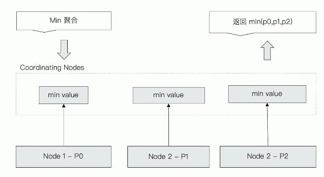
Taking min aggregation as an example, its execution process is shown in the figure below. In fact, it is to find the minimum value of the main partition of three nodes, and finally aggregate it

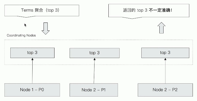
The execution process of terms is shown in the figure below. Now get the first three from each node, and then aggregate the first three from the nine to get the results

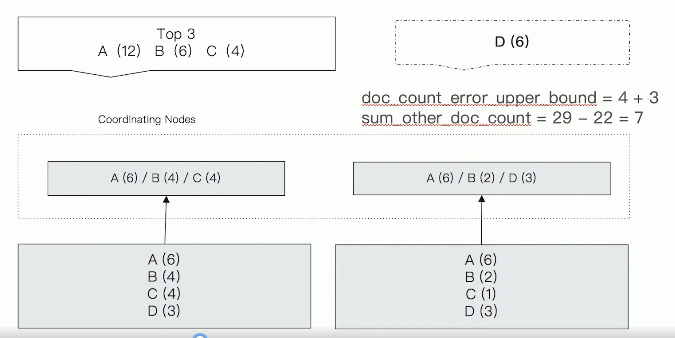
However, the results obtained by this method are not necessarily correct. Please see the following example:

In the above figure, ABC is returned on the left and ABD is returned on the right. After summary, the top three are A(12), B(6) and C(4). However, D actually has 6 documents, which are finally excluded, so an error occurs. In addition, DOC in the figure_ count_ error_ upon_ Bound indicates the maximum number of missing documents in the sub bucket. The maximum number of missing documents in the left sub bucket is 4 and the maximum number of missing documents on the right is 3, so the maximum number of missing documents is 7; And sum_other_doc_count indicates the total number of documents except the final returned documents. In the figure, a total of 12 + 6 + 4 = 22 are returned, then the remaining 7 are returned
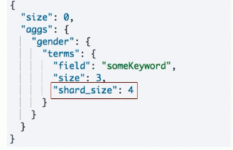
How to solve the problem of inaccurate terms? Set the number of main slices to 1 or increase the shard_size number (so that more data can be obtained from the slice):
