Reference from: Algorithm column
catalogue
3. Comparison of time complexity
1, Time complexity
1. Algorithm efficiency
Evaluation of algorithm efficiency: time complexity and space complexity
Space complexity: the storage space required to execute the program, and the use of computer memory by the algorithm program
Time complexity: it does not mean how much time a program takes to solve a problem, but how fast the length of time required by the program increases when the scale of the problem expands. Measuring the quality of a program depends on how the running time of the program changes after the data scale becomes hundreds of times larger.
The design of algorithm is to first consider the system environment, then weigh the time complexity and space complexity to find a balance point, and the time complexity is often more prone to problems than the space complexity, so the time complexity is the main part of algorithm research and development.
2. Time complexity
Time frequency f(n): the time required for the execution of an algorithm can not be calculated theoretically. It can only be known by computer testing. The execution times of statements in the algorithm are directly proportional to the time spent by the algorithm. More execution times take more time. Therefore, the time complexity is usually calculated by calculating the execution times of statements in the algorithm. The execution times of statements in the algorithm is T(n). N is the scale of the problem. When N changes, T(n) will also change, and the time complexity is the law of this change.
Calculation of time complexity:
In the large o representation, the value of f(n) in O(f(n)) can be 1, N, log(n), n^2 Therefore, O (1), O (n), O (logn) and O (n ^ 2) are called constant order, linear order, logarithmic order and square order respectively.
Rules for deriving the value of f(n):
(1) . replace all addition constants in the number of runs with constant 1
(2).f(n) only the highest order terms are retained
(3) If the highest order term exists and is not 1, remove the constant multiplied by this term
Constant order
  int sum = 0,n = 100; //Execute once
  sum = (1+n)*n/2; //Execute once
  System.out.println (sum); //Execute once
In the above example, f(n)=3. According to rule 1, the time complexity of this algorithm is O(1). If sum = (1+n)*n/2 is executed for another 10 times, the 10 times of execution have nothing to do with the size of N, so the time complexity of the algorithm is still O(1).
Linear order
This paper mainly analyzes the operation of the cycle structure
for(int i=0;i<n;i++){
//Algorithm with time complexity O(1)
...
}
The code in the loop body of the above algorithm has been executed n times, so the time complexity is O(n)
Logarithmic order
int number=1;
while(number<n){
number=number*2;
//Algorithm with time complexity O(1)
...
}
In the above code, each time number is multiplied by 2, it will be closer and closer to N. when number is greater than or equal to N, it will exit the loop. Assuming that the number of cycles is x, x=log n can be obtained from 2^x=n, so the time complexity of this algorithm is O(log n).
Square order
The following code is loop nesting
for(int i=0;i<n;i++){
    for(int j=0;j<n;i++){
       //Algorithm with complexity O(1)
       ...
      }
}
The time complexity of the internal loop code is O(n), and then passes through the external loop n times, so the time complexity of this algorithm is O(n^2).
Let's look at the following algorithm:
  for(int i=0;i<n;i++){
      for(int j=i;j<n;i++){
         //Algorithm with complexity O(1)
         ...
      }
  }
Note that the inner loop becomes j=i, then when i=0, the inner loop is executed n times; When i=1, the inner loop is executed n-1 times; When i=2, the inner loop is executed n-2 times... And so on. The total number of loop executions is:
n+(n-1)+(n-2)+(n-3)+......+1
=(n+1)+[(n-1)+2]+[(n-2)+3]+[(n-3)+4]+......
=(n+1)+(n+1)+(n+1)+(n+1)+......
=(n+1)n/2
=n(n+1)/2
=n²/2+n/2
According to rule 2, only the highest order term and rule 3 remove the constant term, so the time complexity of this algorithm is O(n^2).
3. Comparison of time complexity
In addition to constant order, linear order, square order and logarithmic order, there are the following time complexity:
When f(n)=nlogn, the time complexity is O(nlogn), which can be called nlogn order.
f(n)=n ³ The time complexity is O(n ³), It can be called cubic order.
When f(n)=2 ⁿ, the time complexity is O(2 ⁿ), which can be called exponential order.
When f(n)=n!, the time complexity is O(n!), which can be called factorial order.
When f(n) = (√ n), the time complexity is O(√ n), which can be called square root order.
Algorithms with time complexity of O(n), O(logn), O(√ n) and O(nlogn) do not increase much with the increase of N, so these complexity belong to efficient algorithms; in contrast, O(2 ⁿ) and O(n!) When n increases to 50, the complexity will break through the ten digits. This extremely inefficient complexity is best not to appear in the program. Therefore, it is necessary to evaluate the worst-case complexity of the algorithm when programming.
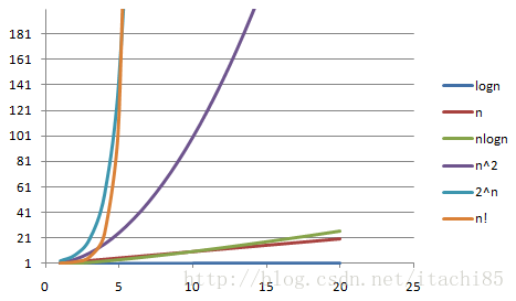
The abscissa is n and the ordinate is T(n). The smaller the change of T(n) with N, the higher the efficiency of the algorithm.
2, Elementary sorting
1. Insert sort
Insert sorting will divide the array to be sorted into two parts, the sorted part and the unordered part. The sorting rule is: treat the beginning element as the sorted part, assign the beginning element to the temporary variable v from the unordered part, move all elements larger than v value back one bit in the sorted part, and insert element v into the empty bit.
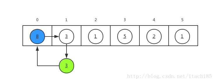
For example, sort array a={8,3,1,5,2,1} from small to large, as shown in the following figure:

Sorting process:
(1) Take a[0]=8 as the sorted part, take out the value of a[1]=3 and assign it to V to obtain v=3, V < a[0], move a[0] backward to a[1], and insert v=3 into the original position of a[0].
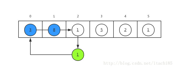
(2).a[0] and a[1] are sorted parts. Assign a[2]=1 to V, and v=1 is less than a[0] and a[1], so move a[1] and a[0] one bit back in turn, and insert v=1 into the position of a[0].
(3) . sort a[3], a[4] and a[5] according to the same rules later.
python code implementation for inserting sorting:
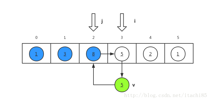
v is the temporary assignment variable, I is the beginning element of the unordered part, and j is the end element of the sorted part. The algorithm idea: the outer loop I increases from 1, and a[i] is assigned to v in each loop; the inner loop decreases from j=i-1, and the sizes of a[j] and v are compared in turn. If it is smaller than v, it moves backward one bit in turn. When j=-1 or a[j] is less than or equal to v, the loop ends.
a = [8, 3, 1, 5, 2, 1]
print('Original sequence:',a)
n = len(a)
for i in range(1, n):
      v = a[i]
      j = i - 1
      while j >= 0 and v < a[j]:
            a[j+1] = a[j]
            j = j - 1
      a[j+1] = v
print('After inserting sorting:',a)


Output results:
Original sequence: [8, 3, 1, 5, 2, 1]
After inserting sorting: [1, 1, 2, 3, 5, 8]
Time complexity of insertion sorting: the optimal time complexity is that the sequence is in ascending order and does not need to be rearranged. At this time, the inner loop complexity is O(1) and the outer loop complexity is O(n), so the optimal time complexity is O(n); the worst time complexity is that when i=1, the inner loop is once, and when i=2, the inner loop is twice until i=n, and the total number of cycles is 1 + 2 + 3 +... + n = n ²/ 2+n/2, the time complexity is O(n^2).
Disadvantages of insert sort: insert sort will only exchange adjacent elements, and elements can only be moved from one end of the array to the other end bit by bit. For large-scale disordered data, insert sort is very slow.
2. Hill sort
Insertion sort is an improved version of insertion sort, that is, the whole sequence is divided into subsequences according to step size, and the subsequences are inserted and sorted. After the whole sequence reaches "basic order", the whole sequence is sorted by insertion sort.
Example: sort [6, 5, 4, 3, 2, 1]
First sorting: the first step is 6 / / 2 = 3
Compare [6, 3]: Exchange [3, 5, 4, 6, 2, 1]
Compare [5, 2]: Exchange [3, 2, 4, 6, 5, 1]
Compare [4, 1]: Exchange [3, 2, 1, 6, 5, 4]
Second sorting: the second step size is 3 / / 2 = 1
Compare [3, 2]: Exchange [2, 3, 1, 6, 5, 4]
Compare [3, 1]: Exchange [2, 1, 3, 6, 5, 4]
Compare [2, 1]: Exchange [1, 2, 3, 6, 5, 4]
Comparison [3, 6]: unchanged [1, 2, 3, 6, 5, 4]
Compare [6, 5]: Exchange [1, 2, 3, 5, 6, 4]
Comparison [3, 5]: unchanged [1, 2, 3, 5, 6, 4]
Comparison [6, 4]: Exchange [1, 2, 3, 5, 4, 6]
Comparison [5, 4]: Exchange [1, 2, 3, 4, 5, 6]
Reference from: Original article by CSDN blogger "Admiral wings of light"
python code implementation of hill sorting:
Algorithm idea (combined with the above example): the outer loop performs insertion sorting by grouping in different steps. In the outer loop, I increases automatically from gap (because the value of J should meet j=i-gap > 0), j=i, and j decreases automatically by step gap in the inner loop. In each loop of I, v is larger than a[j-gap] to perform insertion sorting (only two adjacent elements are exchanged each time), When J is less than gap or v is greater than a[j-gap], the cycle ends.
def shellSort(list_):
      n = len(a)
      gap = n // 2
      while gap > 0:
            for i in range(gap, n):
                  v = list_[i]
                  j = i
                  while j >= gap and v < list_[j-gap]:
                        list_[j] = list_[j-gap]
                        j = j - gap
                  list_[j] = v
            gap = gap // 2
      return list_

a = [9,1,2,5,7,4,8,6,3,5]
print('Original sequence:',a)
a1 = shellSort(a)
print('After sorting:', a1)

Output results:
Original sequence: [9, 1, 2, 5, 7, 4, 8, 6, 3, 5]
After sorting: [1, 2, 3, 4, 5, 5, 6, 7, 8, 9]
Time complexity of hill sorting: Hill sorting is to insert and sort the elements according to the asynchronous length. When the elements are disordered at the beginning, the step size is the largest, so the number of elements inserted and sorted is small and the speed is very fast; When the elements are basically ordered and the step size is very small, insertion sorting is very efficient for ordered sequences. Therefore, the time complexity of Hill sort will be better than O(n^2).
3. Bubble sorting
In each cycle, only adjacent elements are compared from one end to the other. If the order is wrong, they are exchanged. After each cycle, a maximum or minimum value will be obtained, moved to the tail or head end, and the cycle will be repeated until there is no need to exchange again.
The difference between bubble sorting and insertion sorting: after the exchange of adjacent elements, it will continue to proceed regardless of whether the order with the previous elements is correct or not.

python implementation of bubble sorting:
Arrange the sequence from small to large from beginning to end, and divide the array into unordered (front) and sorted (rear) parts. Each cycle of i can arrange a maximum or minimum element, and n-1 cycle is to arrange all elements; j means to compare and sort each unordered element.
def bubbleSort(a):
      n = len(a)
      for i in range(n):
            for j in range(0, n-1-i):
                  if a[j] > a[j+1]:
                        v = a[j+1]
                        a[j+1] = a[j]
                        a[j] = v
      return a

a = [9,1,2,5,7,4,8,6,3,5]
print('Original sequence:',a)
a1 = bubbleSort(a)
print('After bubble sorting:', a1)

Output results:
Original sequence: [9, 1, 2, 5, 7, 4, 8, 6, 3, 5]
After bubble sorting: [1, 2, 3, 4, 5, 5, 6, 7, 8, 9]
4. Quick sort
Select a cardinality and divide the original array into two parts through one-time sorting: the subsequence larger than the cardinality and the subsequence smaller than the cardinality, and then recurse in the subsequence respectively according to the above method. After several times of sorting, the whole sequence becomes orderly
Strategy: divide and conquer, recursion
Implementation process of quick sort (ascending):
(1) For sequence a, select a cardinality x (generally take the first element of the sequence). The leftmost element of the sequence is defined as a[low], low increases from 0, the rightmost element of the sequence is defined as a[high], and high decreases from n-1.
(2) In the first sorting, start from high. If a[high] > x, then high-1; If a[high] < x, assign a[high] to a[low]
(3) Then start from low. If a[low] < x, then low+1; If a[low] > x, assign a[low] to a[high]
(4) Repeat the above steps (2) and (3) from high until high=low
(5) After the first sorting, the subsequence is divided into two parts: the part larger than the base number and the part smaller than the base number. Repeat the above steps (1) ~ (4) in each part respectively until all subsequences are arranged finally.
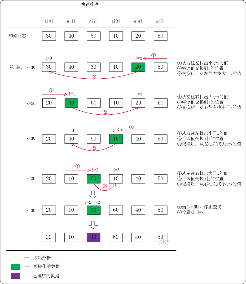
Reference from: Quick sort
Quick sort python code implementation:
def quickSort(a, start, end):
      if start < end:
            low = start
            high = end
            x = a[low]
            while low < high:
                  while low < high and a[high] >= x:
                        high -= 1
                  a[low] = a[high]
                  while low < high and a[low] <= x:
                        low +=1
                  a[high] = a[low]
            a[low] = x
            quickSort(a, start, low-1) #First half recursion
            quickSort(a, high+1, end) #Second half recursion
      return a
a = [3, 4, 6, 1, 2, 5, 7, 1]
print("Before sorting:",a)
n = len(a)
start = 0
end = n-1
a1 = quickSort(a, start, end)
print("After quick sort:",a1)


Output results:
Before sorting: [3, 4, 6, 1, 2, 5, 7, 1]
After quick sort: [1, 1, 2, 3, 4, 5, 6, 7]
Time complexity: the worst time complexity of quick sort is O(n^2), such as the fast arrangement of sequential sequence; The average time complexity is O(nlogn), and the constant factor implicit in the O(nlogn) token is very small, which is much smaller than the merging sort whose complexity is stable equal to O(nlogn). Therefore, for the vast majority of random sequences with weak order, quick sort is always better than merge sort.
5. Merge and sort
Divide and conquer strategy is adopted, including top-down recursion and bottom-up iteration
Merge sorting process:
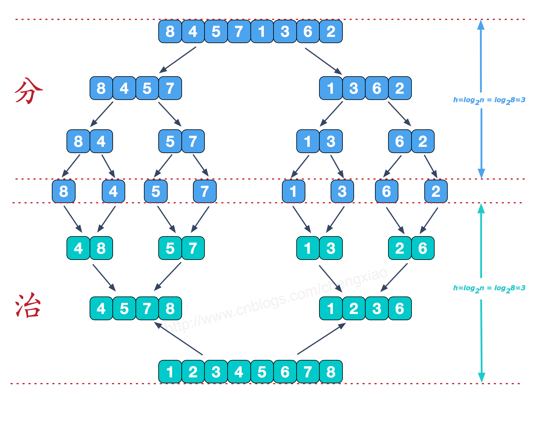
Points:
We divide the original sequence into two small arrays according to 1 / 2 of the sequence length.
2 divide the two small arrays into two smaller ones according to half the new length... Until the sequence is divided into a single element.
For example: 84571362
The first time n=8 n//2=4 is divided into 8457 1362
The second time n=4 n//2=2 divided into 84 57 | 13 62
The third time n=2 n//2=1 is divided into 8 4 5 7 1 3 6 2, which are divided into single elements
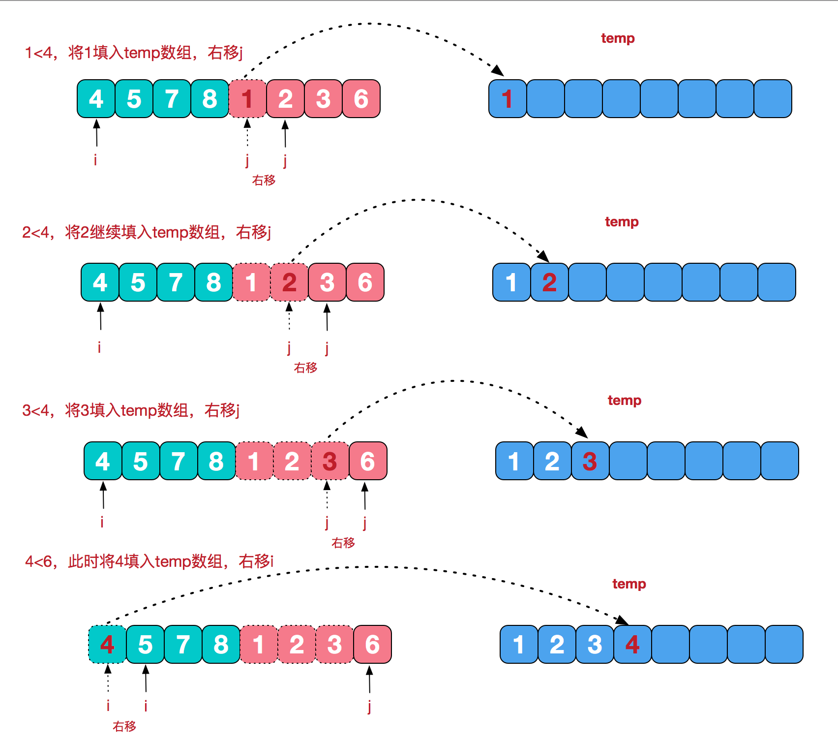
Governance:
3. Compare the size binding of the last two separated elements obtained in step 2 to obtain 48 57 13 26,
4. The obtained subsequences are combined in the order of division to obtain 4578 1236, and then to the final result.
Note: each time, the minimum value of the two arrays is compared, and the minimum value is put into the new array. If one of the last two arrays is put into the new array in advance, just put the remaining array in order.
python implementation of merge sort:
import math
def mergeSort(a):
      n = len(a)
      middle = math.floor(n/2) #math.floor() is rounded down
      if len(a) < 2:
            return a
      else:
            left = a[0 : middle]
            right = a[middle : ]
      return merge(mergeSort(left), mergeSort(right)) #recursion

def merge(left,right):
      '''When neither of the two subsequences is empty, the header elements of the subsequence are compared circularly. When any subsequence is empty, the
      Another subsequence is added to the new sequence in turn'''
      new_a = []
      while left and right: #Neither of the two subsequences is empty
            if left[0] < right[0]:
                  new_a.append(left.pop(0)) #Fetch the data with index 0 and delete it in the original sequence
            else:
                  new_a.append(right.pop(0))
      while left:
            new_a.append(left.pop(0))
      while right:
            new_a.append(right.pop(0))
      return new_a

a = [8, 4, 5, 7, 1, 3, 6, 2]
print('Original sequence:', a)
new_a = mergeSort(a)
print('Merged sequence:', new_a)


Output results:
Original sequence: [8, 4, 5, 7, 1, 3, 6, 2]
Merged sequence: [1, 2, 3, 4, 5, 6, 7, 8]
Time complexity: relatively stable, with a complexity of O(nlogn), but the space complexity is high because a new array has to be created each time.
6. Select sort
First, find the minimum value of the sequence. If it is not in the header element, it will be exchanged with the header element. As a sorted sequence, continue to find the minimum value in all unordered sequences. If it is not in the header element of the unordered sequence, it will be exchanged with the header element and added to the sorted sequence. Cycle until the unordered sequence is empty. 
Select the python implementation for sorting:
First, assume that a[0] is the smallest, and compare the size of a[0] with its subsequent elements. If a[0] is not the smallest, exchange a[0] with the minimum value; Then compare the size of a[1] and its subsequent elements... Until a[n-1].
def selectSort(a):
      n = len(a)
      for i in range(n):
            minnum = i
            for j in range(i, n):
                  if a[j] < a[minnum]:
                        minnum = j #Record the index of the lowest decimal point. Because you don't know where the cycle is the real minimum value, you can't exchange it directly here
            if minnum != i :
                  a[i], a[minnum] = a[minnum], a[i] #exchange
      return a
a = [8, 4, 5, 7, 1, 3, 6, 2]
print('Original sequence:', a)
new_a = selectSort(a)
print('Select the sorted sequence:', new_a)


Output results:
Original sequence: [8, 4, 5, 7, 1, 3, 6, 2]
Select the sorted sequence: [1, 2, 3, 4, 5, 6, 7, 8]
Select the time complexity of sorting: O(n^2)
7. Heap sorting
About heap (from: Heap sorting of graphical sorting algorithm)
Heap is a data structure, also known as complete binary tree, which is divided into large top heap and small top heap.
Large top heap: from top to bottom, the value of each node is greater than or equal to the value of its left and right child nodes.
Small top heap: from top to bottom, the value of each node is less than or equal to the value of its left and right child nodes.
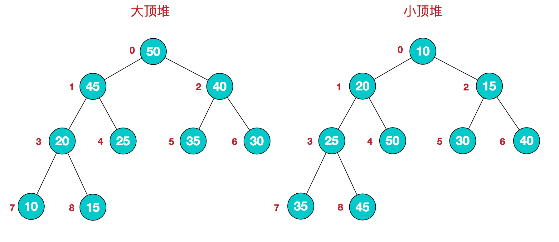
Map this logical structure to the array: large top heap [50,45,40,20,25,35,30,10,15]; small top heap [10,20,15,25,50,30,40,35,45], from top to bottom, from left to right.

Large top reactor
The array is a heap structure in terms of logical structure. The definition of heap structure described by formula is:
Large top pile: arr [i] > = arr [2I + 1] & & arr [i] > = arr [2I + 2]
Small top pile: arr [i] < = arr [2I + 1] & & arr [i] < = arr [2I + 2]
About heap sorting
Heap sorting is to repeat the sequence to construct a complete binary tree according to the definition of the heap, take the maximum or minimum value at the top of the heap and exchange it with the unordered elements of the array, and cycle until it is in order. For example, when constructing an ascending sequence, construct a large top heap from the array, so that the elements at the top of the heap are the maximum value, and exchange this maximum value with arr[n-1]; then reconstruct the large top heap and exchange the elements at the top of the heap with arr[n-2] Swap... Until a[0] completes sorting. (generally, large top heap is used for ascending order and small top heap is used for descending order)
Heap sorting python implementation:
Firstly, in the tree structure, the index value of the last leaf node is n-1, and the index value of the last non leaf node is [(n-1)-1]/2=n/2-1. Heap sorting is realized by recursively calling the heap sorting function.
import math
def heapAdjust(arr, i):
      'Heap adjustment'
      left = 2*i + 1
      right = 2*i + 2
      largest = i
      if left < length and arr[left] > arr[largest]:
            largest = left
      if right < length and arr[right] > arr[largest]:
            largest = right
      if largest != i:
            arr[i], arr[largest] = arr[largest], arr[i] #exchange
            #After an exchange adjustment, you also need to compare whether the adjusted element position and the nodes below it comply with the rules
            heapAdjust(arr, largest)

def maxHeap(arr):
      #Establish initial large top reactor
      for i in range(math.floor(length/2), -1, -1):
            heapAdjust(arr, i)

def heapSort(arr):
      #Heap sort swap element
      global length
      length = len(arr)
      maxHeap(arr)
      for i in range(length-1, 0, -1):
            arr[0], arr[i] = arr[i], arr[0]
            length -= 1
            #After the initial large top heap is constructed, the subsequent sorting can be adjusted from top to bottom
            heapAdjust(arr, 0)
      return arr

arr = [8, 4, 5, 7, 1, 3, 6, 2]
print("Before sorting:", arr)
arr1 = heapSort(arr)
print("After sorting:", arr1)
Time complexity of heap sorting: O(nlogn)
8. Count sorting
(there will be time to reorganize later)