LightGBM
Main advantages of LightGBM:
Easy to use. It provides the mainstream Python\C++\R language interface. Users can easily use LightGBM to model and obtain quite good results.
Efficient and scalable. When dealing with large-scale data sets, it is efficient, fast and accurate, and has low requirements for hardware resources such as memory.
Strong robustness. Compared with the deep learning model, the approximate effect can be achieved without fine tuning.
LightGBM directly supports missing values and category features without additional special processing of data
Main disadvantages of LightGBM:
Compared with the deep learning model, it can not model the space-time position, and can not capture the high-dimensional data such as image, voice, text and so on.
When we have a large amount of training data and can find an appropriate deep learning model, the accuracy of deep learning can be far ahead of LightGBM.
Code flow
Part1 LightGBM classification practice based on hero alliance dataset
Step 1: library function import
Step 2: data reading / loading
Step 3: simple view of data information
Step4: visual description
Step5: training and prediction with LightGBM
Step6: feature selection using LightGBM
Step7: get better results by adjusting parameters
LightGBM classification practice based on hero alliance dataset
At the beginning of practice, we first need to import some basic function libraries, including numpy (the basic software package for scientific computing in Python), pandas (pandas is a fast, powerful, flexible and easy-to-use open source data analysis and processing tool), matplotlib and seaborn drawing.
#Download the data set you need
!wget https://tianchi-media.oss-cn-beijing.aliyuncs.com/DSW/8LightGBM/high_diamond_ranked_10min.csv
step1: function library import
##  Basic function library
import numpy as np
import pandas as pd

## Drawing function library
import matplotlib.pyplot as plt
import seaborn as sns
- Laboratory introduction
1.1 introduction to lightgbm
LightGBM is an extensible machine learning system launched by Microsoft in 2017. It is an open source project of Microsoft's DMKT. It was developed under the leadership of Mr. Ke Guolin, one of the winners of the first Alibaba big data competition in 2014. It is a distributed gradient lifting framework based on GBDT (gradient lifting decision tree) algorithm. In order to meet the needs of shortening the calculation time of the model, the design idea of LightGBM mainly focuses on reducing the use of data on memory and computing performance, as well as reducing the communication cost of multi machine parallel computing.
LightGBM can be regarded as an upgraded luxury version of XGBoost, which not only obtains the accuracy similar to XGBoost, but also provides faster training speed and less memory consumption. As the name of Light implies, LightGBM runs more gracefully and lightly on large-scale data sets. Once launched, it has become a powerful weapon to win the championship in various data competitions.
Main advantages of LightGBM:
Easy to use. It provides the mainstream Python\C++\R language interface. Users can easily use LightGBM to model and obtain quite good results.
Efficient and scalable. When dealing with large-scale data sets, it is efficient, fast and accurate, and has low requirements for hardware resources such as memory.
Strong robustness. Compared with the deep learning model, the approximate effect can be achieved without fine tuning.
LightGBM directly supports missing values and category features without additional special processing of data
Main disadvantages of LightGBM:
Compared with the deep learning model, it can not model the space-time position, and can not capture the high-dimensional data such as image, voice, text and so on.
When we have a large amount of training data and can find an appropriate deep learning model, the accuracy of deep learning can be far ahead of LightGBM.
1.2 application of lightgbm
LightGBM is widely used in the field of machine learning and data mining. According to statistics, LightGBM model has won the top three data competitions on Kaggle platform for more than 30 times from 2016 to 2019, including CIKM2017 AnalytiCup, IEEE Fraud Detection and other well-known competitions. These competitions come from real businesses in all walks of life. These competition results show that LightGBM has good scalability and can achieve very good results on various problems.
At the same time, LightGBM has also been successfully applied to various problems in industry and academia. For example, financial risk control, purchase behavior identification, traffic flow prediction, environmental sound classification, gene classification, biological component analysis and many other fields. Although domain related data analysis and feature engineering also play an important role in these solutions, the consistent choice of LightGBM by learners and practitioners shows the influence and importance of this software package.
- Laboratory Manual
2.1 learning objectives
Understand LightGBM parameters and related knowledge
Master the Python call of LightGBM and apply it to the hero League game victory and defeat prediction data set
2.2 code flow
Part1 LightGBM classification practice based on hero alliance dataset
Step 1: library function import
Step 2: data reading / loading
Step 3: simple view of data information
Step4: visual description
Step5: training and prediction with LightGBM
Step6: feature selection using lightm
Step7: get better results by adjusting parameters
2.3 algorithm practice
2.3.1 LightGBM classification practice based on hero alliance dataset
At the beginning of practice, we first need to import some basic function libraries, including numpy (the basic software package for scientific computing in Python), pandas (pandas is a fast, powerful, flexible and easy-to-use open source data analysis and processing tool), matplotlib and seaborn drawing.
#Download the data set you need
!wget https://tianchi-media.oss-cn-beijing.aliyuncs.com/DSW/8LightGBM/high_diamond_ranked_10min.csv
1
#Download the data set you need
2
!wget https://tianchi-media.oss-cn-beijing.aliyuncs.com/DSW/8LightGBM/high_diamond_ranked_10min.csv
Step 1: function library import
Basic function library
import numpy as np
import pandas as pd
Drawing function library
import matplotlib.pyplot as plt
import seaborn as sns
1
Basic function library
2
import numpy as np
3
import pandas as pd
4
5
Drawing function library
6
import matplotlib.pyplot as plt
7
import seaborn as sns
D:\Software\Anaconda3\lib\site-packages\statsmodels\tools_testing.py:19: FutureWarning: pandas.util.testing is deprecated. Use the functions in the public API at pandas.testing instead.
import pandas.util.testing as tm
This time, we choose the hero alliance dataset for LightGBM scene experience. Hero League is a MOBA competitive online game developed by American fist game in 2009. In each game, the blue team and the red team fight on the same map. The goal of the game is to destroy the defense tower of the enemy team, then destroy the enemy's crystal hub and win the game.
At present, there are 9881 ranking competition data above the diamond segment of hanbok in the League of heroes. The data provides the game status in ten minutes, including the number of kills, the number of deaths, the number of gold coins, experience value, level... And other information. The column blueWins is the label of the data, which represents whether the blue team won the game.
The characteristics of the data are described as follows:
|The name of the feature is the meaning of the feature 124scope of the value range 124124124124124124124124124124124124124124124124124124124124124124124124124124124124124124124124124124124124124124124124124124124124124124124124124124124124124124124124124124124124124124124124124124124124124124124124124124124124124124124124124124124124124124124124124124124124124124\124124124124124124124124124124124124124124124124124\124124124\124124124124\4124124124124124124\124124124124124124124124124integer | Deaths | number of Deaths | integer || The number of Assists is the number of Assists to assist in the number of Assists. The integer 124124124 124124124124 124124124124aroundthe number of large-scale wild monsters to kill and kill the number of large wild monsters 124124 124124 124124124124124 124124124 124124124 124124 124124 124124 124124 124124 124124124 124124 124124124 124124124 124124124124 124124124124124 124124124124124124 124124124124 124124124124124124124124 124124124124124 124124124124124124 124124124124124 \124124124124 \124124124 \4124124124124 \124124124124124124124124124| total economy |||||||||||||||||||||||||||||||||||||124 The hero's total experience is an integral 124124124 124124124 124124124 124124 124124 124124 124124 124124 124124 124124 124 124124 124124\124124 124124124 124124 124124 124 124 124 124 124 124 124124 124 124 124 124124 124 124124124 124124124 124124124 124124124124 124124124124124124 124124124 124124124 124124 124124124 124124124 124124124 \124 124 124 \124 \124124124 \124124124 \124124|||||||||||||||||||||||||||||||||||||
step1: data loading / reading
## We use the read provided by Pandas_ CSV function reads and converts to DataFrame format
df = pd.read_csv('./high_diamond_ranked_10min.csv')
y = df.blueWins

## Use info() view the overall information of the data
df.info()


gameId	blueWins	blueWardsPlaced	blueWardsDestroyed	blueFirstBlood	blueKills	blueDeaths	blueAssists	blueEliteMonsters	blueDragons	...	redTowersDestroyed	redTotalGold	redAvgLevel	redTotalExperience	redTotalMinionsKilled	redTotalJungleMinionsKilled	redGoldDiff	redExperienceDiff	redCSPerMin	redGoldPerMin
0	4519157822	0	28	2	1	9	6	11	0	0	...	0	16567	6.8	17047	197	55	-643	8	19.7	1656.7
1	4523371949	0	12	1	0	5	5	5	0	0	...	1	17620	6.8	17438	240	52	2908	1173	24.0	1762.0
2	4521474530	0	15	0	0	7	11	4	1	1	...	0	17285	6.8	17254	203	28	1172	1033	20.3	1728.5
3	4524384067	0	43	1	0	4	5	5	1	0	...	0	16478	7.0	17961	235	47	1321	7	23.5	1647.8
4	4436033771	0	75	4	0	6	6	6	0	0	...	0	17404	7.0	18313	225	67	1004	-230	22.5	1740.4
,
The number of positive and negative labels of the data set is basically the same, and there is no problem of data imbalance.
## Dimension feature column
drop_cols = ['gameId','blueWins']
x = df.drop(drop_cols, axis=1)

## Make some statistical description for the characteristics
x.describe()

blueWardsPlaced	blueWardsDestroyed	blueFirstBlood	blueKills	blueDeaths	blueAssists	blueEliteMonsters	blueDragons	blueHeralds	blueTowersDestroyed	...	redTowersDestroyed	redTotalGold	redAvgLevel	redTotalExperience	redTotalMinionsKilled	redTotalJungleMinionsKilled	redGoldDiff	redExperienceDiff	redCSPerMin	redGoldPerMin
count	9879.000000	9879.000000	9879.000000	9879.000000	9879.000000	9879.000000	9879.000000	9879.000000	9879.000000	9879.000000	...	9879.000000	9879.000000	9879.000000	9879.000000	9879.000000	9879.000000	9879.000000	9879.000000	9879.000000	9879.000000
mean	22.288288	2.824881	0.504808	6.183925	6.137666	6.645106	0.549954	0.361980	0.187974	0.051422	...	0.043021	16489.041401	6.925316	17961.730438	217.349226	51.313088	-14.414111	33.620306	21.734923	1648.904140
std	18.019177	2.174998	0.500002	3.011028	2.933818	4.064520	0.625527	0.480597	0.390712	0.244369	...	0.216900	1490.888406	0.305311	1198.583912	21.911668	10.027885	2453.349179	1920.370438	2.191167	149.088841
min	5.000000	0.000000	0.000000	0.000000	0.000000	0.000000	0.000000	0.000000	0.000000	0.000000	...	0.000000	11212.000000	4.800000	10465.000000	107.000000	4.000000	-11467.000000	-8348.000000	10.700000	1121.200000
25%	14.000000	1.000000	0.000000	4.000000	4.000000	4.000000	0.000000	0.000000	0.000000	0.000000	...	0.000000	15427.500000	6.800000	17209.500000	203.000000	44.000000	-1596.000000	-1212.000000	20.300000	1542.750000
50%	16.000000	3.000000	1.000000	6.000000	6.000000	6.000000	0.000000	0.000000	0.000000	0.000000	...	0.000000	16378.000000	7.000000	17974.000000	218.000000	51.000000	-14.000000	28.000000	21.800000	1637.800000
75%	20.000000	4.000000	1.000000	8.000000	8.000000	9.000000	1.000000	1.000000	0.000000	0.000000	...	0.000000	17418.500000	7.200000	18764.500000	233.000000	57.000000	1585.500000	1290.500000	23.300000	1741.850000
max	250.000000	27.000000	1.000000	22.000000	22.000000	29.000000	2.000000	1.000000	1.000000	4.000000	...	2.000000	22732.000000	8.200000	22269.000000	289.000000	92.000000	10830.000000	9333.000000	28.900000	2273.200000
We found that there was a significant difference between the value range of the number of inserted eyes and the number of removed eyes in different games, and there was even an abnormal value of 250 inserted eyes in the first ten minutes.
We found that the value of EliteMonsters is equivalent to Deagons + Heralds.
We found that variables such as TotalGold had little difference in most matches.
We found that the economic difference and experience difference of the two teams are opposite.
We found that the probability of red team and blue team getting the first kill is about 50%
## According to the above description, we can remove some duplicate variables. For example, as long as we know whether the blue team gets a blood, we will know whether the red team has got it, and we can remove the relevant redundant data of the red team.
drop_cols = ['redFirstBlood','redKills','redDeaths'
             ,'redGoldDiff','redExperienceDiff', 'blueCSPerMin',
            'blueGoldPerMin','redCSPerMin','redGoldPerMin']
x.drop(drop_cols, axis=1, inplace=True)
Step4: visual description
data = x
data_std = (data - data.mean()) / data.std()
data = pd.concat([y, data_std.iloc[:, 0:9]], axis=1)
data = pd.melt(data, id_vars='blueWins', var_name='Features', value_name='Values')

fig, ax = plt.subplots(1,2,figsize=(15,5))

# Drawing violin
sns.violinplot(x='Features', y='Values', hue='blueWins', data=data, split=True,
               inner='quart', ax=ax[0], palette='Blues')
fig.autofmt_xdate(rotation=45)

data = x
data_std = (data - data.mean()) / data.std()
data = pd.concat([y, data_std.iloc[:, 9:18]], axis=1)
data = pd.melt(data, id_vars='blueWins', var_name='Features', value_name='Values')

# Drawing violin
sns.violinplot(x='Features', y='Values', hue='blueWins',
               data=data, split=True, inner='quart', ax=ax[1], palette='Blues')
fig.autofmt_xdate(rotation=45)

plt.show()
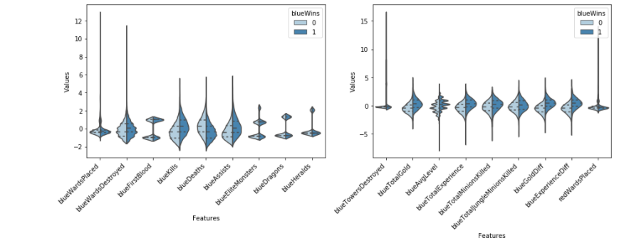
Violin plot is used to show the distribution status and probability density of multiple groups of data. This kind of chart combines the characteristics of box chart and density chart, and is mainly used to show the distribution shape of data.
As can be seen from the figure:
The more heroes killed, the easier it is to win, and the more deaths, the easier it is to lose (the difference between blue kills and blue deaths).
The number of assists is similar to the figure formed by the number of heroes killed, indicating that they have almost the same impact on the result of the game.
The achievement of one blood has a positive correlation with winning, but the correlation is not as obvious as the number of heroes killed.
Poor economy and experience have a great impact on the outcome of the game.
The number of wild monsters killed has little effect on the outcome of the game.
plt.figure(figsize=(18,14))
sns.heatmap(round(x.corr(),2), cmap='Blues', annot=True)
plt.show()
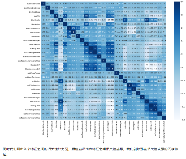
# Remove redundant features
drop_cols = ['redAvgLevel','blueAvgLevel']
x.drop(drop_cols, axis=1, inplace=True)
sns.set(style='whitegrid', palette='muted')

# Two new features of structure
x['wardsPlacedDiff'] = x['blueWardsPlaced'] - x['redWardsPlaced']
x['wardsDestroyedDiff'] = x['blueWardsDestroyed'] - x['redWardsDestroyed']

data = x[['blueWardsPlaced','blueWardsDestroyed','wardsPlacedDiff','wardsDestroyedDiff']].sample(1000)
data_std = (data - data.mean()) / data.std()
data = pd.concat([y, data_std], axis=1)
data = pd.melt(data, id_vars='blueWins', var_name='Features', value_name='Values')

plt.figure(figsize=(10,6))
sns.swarmplot(x='Features', y='Values', hue='blueWins', data=data)
plt.xticks(rotation=45)
plt.show()
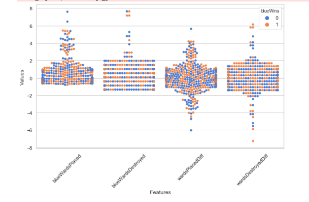
We draw a scatter diagram of the number of holes inserted and find that there is no significant law between the number of holes inserted and the outcome of the game. It is speculated that the number of holes inserted and pulled out in the first ten minutes in the data has little impact on the game, because it is a routine to insert and arrange the holes above the diamond segment. So let's remove these features for the time being.
## Remove features related to eye position
drop_cols = ['blueWardsPlaced','blueWardsDestroyed','wardsPlacedDiff',
            'wardsDestroyedDiff','redWardsPlaced','redWardsDestroyed']
x.drop(drop_cols, axis=1, inplace=True)
x['killsDiff'] = x['blueKills'] - x['blueDeaths']
x['assistsDiff'] = x['blueAssists'] - x['redAssists']

x[['blueKills','blueDeaths','blueAssists','killsDiff','assistsDiff','redAssists']].hist(figsize=(12,10), bins=20)
plt.show()
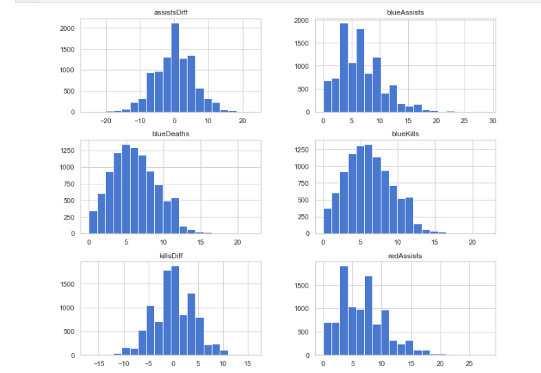
We found that there was little difference in the data distribution of kills, deaths and assists. However, the distribution of kill minus death and assist minus death is very different from the original distribution, so we newly construct these two characteristics.
data = x[['blueKills','blueDeaths','blueAssists','killsDiff','assistsDiff','redAssists']].sample(1000)
data_std = (data - data.mean()) / data.std()
data = pd.concat([y, data_std], axis=1)
data = pd.melt(data, id_vars='blueWins', var_name='Features', value_name='Values')

plt.figure(figsize=(10,6))
sns.swarmplot(x='Features', y='Values', hue='blueWins', data=data)
plt.xticks(rotation=45)
plt.show()
From the above figure, we can find that the number of kills, deaths and assists, as well as the features we constructed have good classification ability for the data.
data = pd.concat([y, x], axis=1).sample(500)

sns.pairplot(data, vars=['blueKills','blueDeaths','blueAssists','killsDiff','assistsDiff','redAssists'],
             hue='blueWins')

plt.show()
After some features are combined in pairs, the data division ability is also improved.
x['dragonsDiff'] = x['blueDragons'] - x['redDragons']
x['heraldsDiff'] = x['blueHeralds'] - x['redHeralds']
x['eliteDiff'] = x['blueEliteMonsters'] - x['redEliteMonsters']

data = pd.concat([y, x], axis=1)

eliteGroup = data.groupby(['eliteDiff'])['blueWins'].mean()
dragonGroup = data.groupby(['dragonsDiff'])['blueWins'].mean()
heraldGroup = data.groupby(['heraldsDiff'])['blueWins'].mean()

fig, ax = plt.subplots(1,3, figsize=(15,4))

eliteGroup.plot(kind='bar', ax=ax[0])
dragonGroup.plot(kind='bar', ax=ax[1])
heraldGroup.plot(kind='bar', ax=ax[2])

print(eliteGroup)
print(dragonGroup)
print(heraldGroup)

plt.show()
We constructed the difference between the two teams in the number of whether to get the dragon, whether to get the canyon pioneer and kill large wild monsters. We found that getting the dragon in the early stage of the game is easier to win than getting the canyon pioneer. There is also a strong correlation between the number of large wild monsters and the winning rate.
x['towerDiff'] = x['blueTowersDestroyed'] - x['redTowersDestroyed']

data = pd.concat([y, x], axis=1)

towerGroup = data.groupby(['towerDiff'])['blueWins']
print(towerGroup.count())
print(towerGroup.mean())

fig, ax = plt.subplots(1,2,figsize=(15,5))

towerGroup.mean().plot(kind='line', ax=ax[0])
ax[0].set_title('Proportion of Blue Wins')
ax[0].set_ylabel('Proportion')

towerGroup.count().plot(kind='line', ax=ax[1])
ax[1].set_title('Count of Towers Destroyed')
ax[1].set_ylabel('Count')
Twitter is the core of the League of Heroes game, so the number of twitter may have a lot to do with the outcome of the game. We found that although the probability of pushing down the first defense tower in the first ten minutes is very low, once a team pushes down the first defense tower, the winning rate of the game will greatly increase.
Step5: training and prediction with LightGBM
## In order to correctly evaluate the performance of the model, the data is divided into training set and test set, the model is trained on the training set, and the performance of the model is verified on the test set.
from sklearn.model_selection import train_test_split

## Select samples with categories 0 and 1 (excluding samples with category 2)
data_target_part = y
data_features_part = x

## The test set size is 20%, 80% / 20% points
x_train, x_test, y_train, y_test = train_test_split(data_features_part, data_target_part, test_size = 0.2, random_state = 2020)
## Import LightGBM model
from lightgbm.sklearn import LGBMClassifier
## Define LightGBM model
clf = LGBMClassifier()
# Training LightGBM model on training set
clf.fit(x_train, y_train)
## The distribution on the training set and test set is predicted by using the trained model
train_predict = clf.predict(x_train)
test_predict = clf.predict(x_test)
from sklearn import metrics

## The model effect is evaluated by accuracy [the proportion of the number of correctly predicted samples to the total number of predicted samples]
print('The accuracy of the Logistic Regression is:',metrics.accuracy_score(y_train,train_predict))
print('The accuracy of the Logistic Regression is:',metrics.accuracy_score(y_test,test_predict))

## View the confusion matrix (statistical matrix of various situations of predicted value and real value)
confusion_matrix_result = metrics.confusion_matrix(test_predict,y_test)
print('The confusion matrix result:\n',confusion_matrix_result)

# Visualization of results using thermal maps
plt.figure(figsize=(8, 6))
sns.heatmap(confusion_matrix_result, annot=True, cmap='Blues')
plt.xlabel('Predicted labels')
plt.ylabel('True labels')
plt.show()
We can find that a total of 718 + 707 samples are predicted correctly and 306 + 245 samples are predicted incorrectly.
Step7: feature selection using LightGBM
The feature selection of LightGBM belongs to the embedded method in feature selection, and the attribute feature can be used in LightGBM_ importances_ To see the importance of the feature.
sns.barplot(y=data_features_part.columns, x=clf.feature_importances_)
The characteristics such as the total economic gap, the number of assists and the number of killed people all play a great role. The number of inserted holes and the number of push towers have little effect on the model.
In addition to the first time, we can also use the following important attributes in LightGBM to evaluate the importance of features.
gain: evaluation Gini index when using features for division
split: it is evaluated by the number of times the feature is used
from sklearn.metrics import accuracy_score
from lightgbm import plot_importance

def estimate(model,data):

    #sns.barplot(data.columns,model.feature_importances_)
    ax1=plot_importance(model,importance_type="gain")
    ax1.set_title('gain')
    ax2=plot_importance(model, importance_type="split")
    ax2.set_title('split')
    plt.show()
def classes(data,label,test):
    model=LGBMClassifier()
    model.fit(data,label)
    ans=model.predict(test)
    estimate(model, data)
    return ans

ans=classes(x_train,y_train,x_test)
pre=accuracy_score(y_test, ans)
print('acc=',accuracy_score(y_test,ans))
These diagrams can also help us better understand other important features
Step8: get better results by adjusting parameters
LightGBM includes but is not limited to the following parameters that have a great impact on the model:
learning_rate: sometimes called eta. The default value is 0.3. The step size of each iteration is very important. It is too large, the operation accuracy is not high, and it is too small, and the operation speed is slow.
num_leaves: 32 by default. This parameter controls the maximum number of leaf nodes in each tree.
feature_fraction: the default value is 1. We usually set it to about 0.8. It is used to control the proportion of the number of columns sampled randomly per tree (each column is a feature).
max_depth: the default value of the system is 6. We often use a number between 3 and 10. This value is the maximum depth of the tree. This value is used to control over fitting. max_ The greater the depth, the more specific the model learning.
The methods of adjusting model parameters include greedy algorithm, grid parameter adjustment, Bayesian parameter adjustment and so on. Here we use grid parameter adjustment. Its basic idea is exhaustive search: in all candidate parameter selection, try every possibility through cyclic traversal, and the best parameter is the final result.
## Import grid parameter adjustment function from sklearn Library
from sklearn.model_selection import GridSearchCV

## Define parameter value range
learning_rate = [0.1, 0.3, 0.6]
feature_fraction = [0.5, 0.8, 1]
num_leaves = [16, 32, 64]
max_depth = [-1,3,5,8]

parameters = { 'learning_rate': learning_rate,
              'feature_fraction':feature_fraction,
              'num_leaves': num_leaves,
              'max_depth': max_depth}
model = LGBMClassifier(n_estimators = 50)

## Perform grid search
clf = GridSearchCV(model, parameters, cv=3, scoring='accuracy',verbose=3, n_jobs=-1)
clf = clf.fit(x_train, y_train)
## The best parameters after grid search are

clf.best_params_
## The best model parameters are used to predict the distribution on the training set and test set

## Define LightGBM model with parameters
clf = LGBMClassifier(feature_fraction = 0.8,
                    learning_rate = 0.1,
                    max_depth= 3,
                    num_leaves = 16)
# Training LightGBM model on training set
clf.fit(x_train, y_train)

train_predict = clf.predict(x_train)
test_predict = clf.predict(x_test)

## The model effect is evaluated by accuracy [the proportion of the number of correctly predicted samples to the total number of predicted samples]
print('The accuracy of the Logistic Regression is:',metrics.accuracy_score(y_train,train_predict))
print('The accuracy of the Logistic Regression is:',metrics.accuracy_score(y_test,test_predict))

## View the confusion matrix (statistical matrix of various situations of predicted value and real value)
confusion_matrix_result = metrics.confusion_matrix(test_predict,y_test)
print('The confusion matrix result:\n',confusion_matrix_result)

# Visualization of results using thermal maps
plt.figure(figsize=(8, 6))
sns.heatmap(confusion_matrix_result, annot=True, cmap='Blues')
plt.xlabel('Predicted labels')
plt.ylabel('True labels')
plt.show()
Originally, there were 306 + 245 errors, but now there are 287 + 230 errors, which has significantly improved the accuracy.
Important knowledge points
2.4.1 important parameters of lightgbm
2.4.1.1 basic parameter adjustment
num_leaves parameter, which is the main parameter to control the complexity of the tree model. Generally, we will make num_leaves is less than (max_depth power of 2) to prevent over fitting. LightGBM is a leaf wise tree, which is different from XGBoost's depth wise tree building method, num_leaves is more effective than depth
min_data_in_leaf this is a very important parameter in dealing with the over fitting problem Its value depends on the sample tree and num of the training data_ Leaves parameter Setting it larger can avoid generating a too deep tree, but it may lead to under fitting In practical application, for large data sets, setting it to hundreds or thousands is enough
max_depth of depth tree. The concept of depth does not play a big role in leaf wise tree, because there is no reasonable mapping from leaves to depth.
2.4.1.2 parameter adjustment for training speed
By setting bagging_fraction and bagging_ Use the bagging method with the freq parameter.
By setting the feature_fraction parameter to use subsampling of features.
Choose a smaller max_bin parameter.
Using save_binary will accelerate data loading in the future learning process.
2.4.1.3 parameter adjustment for accuracy
Use a larger max_bin (learning speed may slow down)
Use smaller learning_rate and larger num_iterations
Use larger num_leaves (may cause overfitting)
Use larger training data
Try dart mode
2.4.1.4 parameter adjustment for over fitting
Use smaller max_bin
Use smaller num_leaves
Use min_data_in_leaf and min_sum_hessian_in_leaf
By setting bagging_fraction and bagging_freq to use bagging
By setting the feature_fraction to use feature subsampling
Use larger training data
Using lambda_l1, lambda_l2 and min_gain_to_split to use regular
Try max_depth to avoid generating too deep trees
2.4.2 rough explanation of lightgbm principle
The bottom layer of LightGBM implements GBDT algorithm and adds a series of new features:
The optimization based on histogram algorithm makes the data storage more convenient, the operation faster, the robustness stronger and the model more stable.
A leaf wise algorithm with depth constraints is proposed, which abandons the level wise decision tree growth strategy used by most GBDT tools and uses the leaf growth strategy with depth constraints, which can reduce the error and obtain better accuracy.
A unilateral gradient sampling algorithm is proposed, which excludes most small gradient samples and uses only the remaining samples to calculate the information gain. It is an algorithm that balances the amount of data and accuracy.
A mutually exclusive feature binding algorithm is proposed. The high-dimensional data is often sparse. This sparsity inspires us to design a lossless method to reduce the dimension of features. Usually, the bundled features are mutually exclusive (that is, the features will not be non-zero at the same time, such as one hot), so that the two features will not lose information when they are bundled.
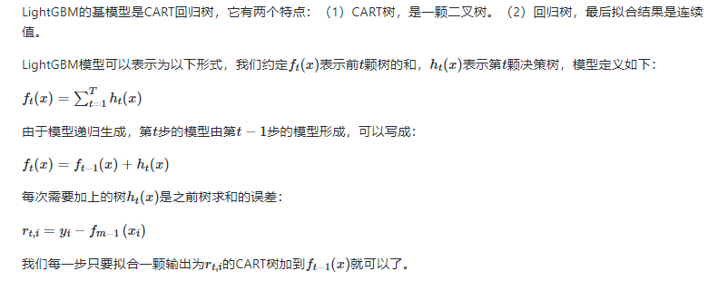
LightGBM is an integrated model based on CART tree. Its idea is to connect multiple decision tree models in series to make decisions together.
image.png
So how to connect in series? LightGBM adopts the method of iterative prediction error. As a popular example, we now need to predict the value of a car at 3000 yuan. We build decision tree 1. After training, the prediction is 2600 yuan. We find that there is an error of 400 yuan, so the training goal of decision tree 2 is 400 yuan, but the prediction result of decision tree 2 is 350 yuan. If there is still an error of 50 yuan, we will give it to the third tree... And so on. Each tree is used to estimate the error of all previous trees. Finally, the sum of the prediction results of all trees is the final prediction result!
end