Project background
Taking the behavior data of an e-commerce user as the data set, this data report analyzes the behavior of Taobao users through industry indicators, so as to explore the behavior mode of an e-commerce user. The specific indicators include daily PV and daily UV analysis, payment rate analysis, funnel loss analysis and user price RFM analysis.
Understanding data
This data set is the user behavior data of an e-commerce from November 18, 2014 to December 18, 2014, with a total of 6 columns of fields, which are:
user_id: user identity, desensitization
item_id: Commodity ID, desensitization
behavior_type: user behavior type (including clicking, collecting, adding shopping cart and paying, represented by numbers 1, 2, 3 and 4 respectively)
user_geohash: geographic location
item_category: category ID (category to which the commodity belongs)
Time: the time when the user behavior occurs
Data cleaning
import pandas as pd
import numpy as np
import matplotlib.pyplot as plt
import seaborn as sns
# Remove the display of warning log reminder
from pandas.plotting import register_matplotlib_converters
register_matplotlib_converters()
#Solve the display problems such as Chinese garbled code
%matplotlib inline
plt.rcParams['font.sans-serif']=['SimHei']
plt.rcParams['axes.unicode_minus']=False
%config InlineBackend.figure_format = 'svg'
data = pd.read_csv(r"D:\study\Data analysis project\Taobao user behavior analysis\tianchi_mobile_recommend_train_user\tianchi_mobile_recommend_train_user.csv")
data.head()
| user_id | item_id | behavior_type | user_geohash | item_category | time | |
|---|---|---|---|---|---|---|
| 0 | 98047837 | 232431562 | 1 | NaN | 4245 | 2014-12-06 02 |
| 1 | 97726136 | 383583590 | 1 | NaN | 5894 | 2014-12-09 20 |
| 2 | 98607707 | 64749712 | 1 | NaN | 2883 | 2014-12-18 11 |
| 3 | 98662432 | 320593836 | 1 | 96nn52n | 6562 | 2014-12-06 10 |
| 4 | 98145908 | 290208520 | 1 | NaN | 13926 | 2014-12-16 21 |
Missing value processing
data.isnull().sum()
user_id                0
item_id                0
behavior_type          0
user_geohash     8334824
item_category          0
time                   0
dtype: int64
data.fillna('miss',inplace=True)
Standardized treatment
#Split dataset
import re
data['date'] = data['time'].map(lambda s: re.compile(' ').split(s)[0])
data['hour'] = data['time'].map(lambda s: re.compile(' ').split(s)[1])
data.head()
| user_id | item_id | behavior_type | user_geohash | item_category | time | date | hour | |
|---|---|---|---|---|---|---|---|---|
| 0 | 98047837 | 232431562 | 1 | miss | 4245 | 2014-12-06 02 | 2014-12-06 | 02 |
| 1 | 97726136 | 383583590 | 1 | miss | 5894 | 2014-12-09 20 | 2014-12-09 | 20 |
| 2 | 98607707 | 64749712 | 1 | miss | 2883 | 2014-12-18 11 | 2014-12-18 | 11 |
| 3 | 98662432 | 320593836 | 1 | 96nn52n | 6562 | 2014-12-06 10 | 2014-12-06 | 10 |
| 4 | 98145908 | 290208520 | 1 | miss | 13926 | 2014-12-16 21 | 2014-12-16 | 21 |
data.dtypes
user_id           int64
item_id           int64
behavior_type     int64
user_geohash     object
item_category     int64
time             object
date             object
hour             object
dtype: object
#Convert the time column and date column into date data type, and the hour column should be string data type.
#Data type conversion
data['date']=pd.to_datetime(data['date'])
data['time']=pd.to_datetime(data['time'])
data['hour']=data['hour'].astype('int64')
data.dtypes
user_id                   int64
item_id                   int64
behavior_type             int64
user_geohash             object
item_category             int64
time             datetime64[ns]
date             datetime64[ns]
hour                      int64
dtype: object
data = data.sort_values(by='time',ascending=True)#Sorting processing
data = data.reset_index(drop=True)#Indexing
data
| user_id | item_id | behavior_type | user_geohash | item_category | time | date | hour | |
|---|---|---|---|---|---|---|---|---|
| 0 | 73462715 | 378485233 | 1 | miss | 9130 | 2014-11-18 00:00:00 | 2014-11-18 | 0 |
| 1 | 36090137 | 236748115 | 1 | miss | 10523 | 2014-11-18 00:00:00 | 2014-11-18 | 0 |
| 2 | 40459733 | 155218177 | 1 | miss | 8561 | 2014-11-18 00:00:00 | 2014-11-18 | 0 |
| 3 | 814199 | 149808524 | 1 | miss | 9053 | 2014-11-18 00:00:00 | 2014-11-18 | 0 |
| 4 | 113309982 | 5730861 | 1 | miss | 3783 | 2014-11-18 00:00:00 | 2014-11-18 | 0 |
| ... | ... | ... | ... | ... | ... | ... | ... | ... |
| 12256901 | 132653097 | 119946062 | 2 | miss | 6054 | 2014-12-18 23:00:00 | 2014-12-18 | 23 |
| 12256902 | 130082553 | 296196819 | 1 | miss | 11532 | 2014-12-18 23:00:00 | 2014-12-18 | 23 |
| 12256903 | 43592945 | 350594832 | 1 | 9rhhgph | 9541 | 2014-12-18 23:00:00 | 2014-12-18 | 23 |
| 12256904 | 12833799 | 186993938 | 1 | 954g37v | 3798 | 2014-12-18 23:00:00 | 2014-12-18 | 23 |
| 12256905 | 77522552 | 69292191 | 1 | miss | 889 | 2014-12-18 23:00:00 | 2014-12-18 | 23 |
12256906 rows × 8 columns
User behavior analysis
PV (traffic): that is, Page View, specifically refers to the page views or clicks of the website, which is calculated once the page is refreshed.
UV (independent visitor): that is, Unique Visitor. A computer client accessing the website is a visitor.
Daily traffic analysis
#pv_daily records the number of user operations per day, uv_daily records the number of different online users every day
pv_daily = data.groupby('date')['user_id'].count().reset_index().rename(columns={'user_id':'pv'})
uv_daily = data.groupby('date')['user_id'].apply(lambda x:x.drop_duplicates().count()).reset_index().rename(columns={'user_id':'uv'})
fig,axes=plt.subplots(2,1)
pv_daily.plot(x='date',y='pv',ax=axes[0])
uv_daily.plot(x='date',y='uv',ax=axes[1])
axes[0].set_title('pv_daily')
axes[1].set_title('uv_daily')

plt.show()
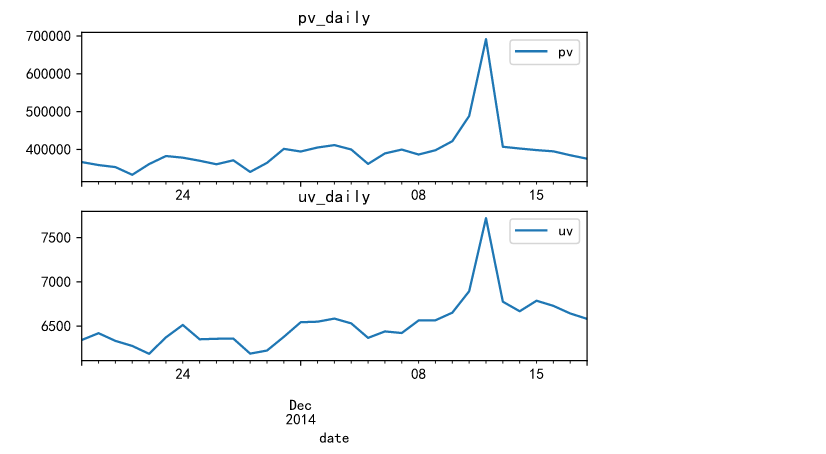
The results show that, as shown in the above figure, the pv and uv traffic reaches the peak value during the double twelve, and it can be found that there is a large gap between the uv and pv traffic values.
Hourly traffic analysis
#pv_hour records the number of user operations per hour, UV_ Number of online users per hour
pv_hour = data.groupby('hour')['user_id'].count().reset_index().rename(columns={'user_id':'pv'})
uv_hour = data.groupby('hour')['user_id'].apply(lambda x:x.drop_duplicates().count()).reset_index().rename(columns={'user_id':'uv'})
fig,axes = plt.subplots(2,1,sharex=True)
pv_hour.plot(x='hour',y='pv',ax=axes[0])
uv_hour.plot(x='hour',y='uv',ax=axes[1])
axes[0].set_title('pv_hour')
axes[1].set_title('uv_hour')
plt.show()
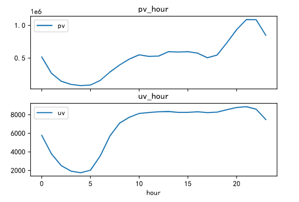
The fluctuation of pv and uv is the same during 0-5 a.m., and both show a downward trend. The traffic reaches the lowest point at 5 a.m. at the same time, at about 18:00 p.m., the fluctuation of pv is relatively intense. Compared with uv, it is not obvious. It can be seen that after 18:00 p.m., it is the active time period for Taobao users to visit the app.
pv analysis of users with different behavior types
pv_detail = data.groupby(['behavior_type','hour'])['user_id'].count().reset_index().rename(columns={'user_id':'total_pv'})
fig,axes = plt.subplots(2,1,sharex=True)
sns.pointplot(x='hour',y='total_pv',hue='behavior_type',data=pv_detail,ax=axes[0])
sns.pointplot(x='hour',y='total_pv',hue='behavior_type',data=pv_detail[pv_detail.behavior_type!=1],ax=axes[1])

axes[0].set_title('pv_different_behavior_type')
plt.show()
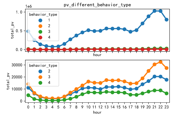
The chart shows that compared with the other three types of user behaviors, the click user behavior has higher pv visits, and the fluctuations of the four user behaviors are basically the same. Therefore, no matter which user behavior is at night, the pv visits are the highest.
Consumer behavior analysis
Analysis of user purchase times
data_buy=data[data.behavior_type==4].groupby('user_id')['behavior_type'].count()
sns.displot(data_buy)
plt.title('daily_buy')
plt.show()
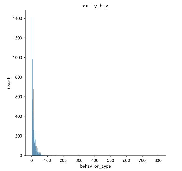
data_buy=data[data.behavior_type==4].groupby('user_id')['behavior_type'].count().reset_index().rename(columns={'behavior_type':'buy_count'})
data_buy.describe()
| user_id | buy_count | |
|---|---|---|
| count | 8.886000e+03 | 8886.000000 |
| mean | 7.152087e+07 | 13.527459 |
| std | 4.120719e+07 | 19.698786 |
| min | 4.913000e+03 | 1.000000 |
| 25% | 3.567731e+07 | 4.000000 |
| 50% | 7.238800e+07 | 8.000000 |
| 75% | 1.071945e+08 | 17.000000 |
| max | 1.424559e+08 | 809.000000 |
bins = [1,10,20,50]
data_buy['buy_count_cut'] = pd.cut(data_buy['buy_count'],bins,labels = ['1-10','10-20','20-50'])
buy_count_cut = data_buy['buy_count_cut'].value_counts()
buy_count_cut
1-10     4472
10-20    1972
20-50    1417
Name: buy_count_cut, dtype: int64
Taobao users generally spend less than 10 times, so we need to focus on the consumer user groups who buy more than 10 times.
Rate
Payment rate = number of consumers / number of active users
data.groupby('date').apply(lambda x:x[x.behavior_type==4].count()/len(x.user_id.unique())).plot()
plt.title('Rate ')
Text(0.5, 1.0, 'Rate ')
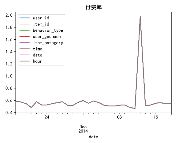
About 6% of the daily active users have consumption behavior, with the largest number of users during the double 12.
Funnel loss analysis
Browse the home page - click on products - add to shopping cart & collection - start payment - complete purchase
data_user = data.groupby(['behavior_type']).count()
data_user.head()
| user_id | item_id | user_geohash | item_category | time | date | hour | |
|---|---|---|---|---|---|---|---|
| behavior_type | |||||||
| 1 | 11550581 | 11550581 | 11550581 | 11550581 | 11550581 | 11550581 | 11550581 |
| 2 | 242556 | 242556 | 242556 | 242556 | 242556 | 242556 | 242556 |
| 3 | 343564 | 343564 | 343564 | 343564 | 343564 | 343564 | 343564 |
| 4 | 120205 | 120205 | 120205 | 120205 | 120205 | 120205 | 120205 |
pv_all=data['user_id'].count()
print(pv_all)
12256906
Total views: 12256906
Hits: 11550581
Collection quantity + additional purchase quantity: 242556 + 343564 = 586120
Purchase volume: 120205
Number of hits - loss rate of purchase intention: 94.93%
Purchase intention - loss rate of purchase volume: 79.49%
In this data set, there is a lack of user behavior data of "placing orders", so it is impossible to analyze the turnover rate from placing orders to the completion of final payment.
At the same time, because there is no superior subordinate relationship between the two user behaviors of collection and additional purchase, they are combined into purchase intention for analysis.
Analysis of user value RFM model
Meaning of RFM:
R(Recency): The interval between the last transaction of the customer. R The larger the value, the longer the date of customer transaction; otherwise, the closer the date of customer transaction.
F(Frequency): The number of transactions the customer has made in the recent period. F The higher the value, the more frequent the customer transactions; otherwise, the less active the customer transactions.
M(Monetary): The amount of the customer's transaction in the latest period of time. M The higher the value, the higher the customer value; otherwise, the lower the customer value.
from datetime import datetime
datenow=datetime(2014,12,20)
#Latest purchase time per user
recent_buy_time=data[data.behavior_type==4].groupby('user_id').date.apply(lambda x:datetime(2014,12,20)-x.sort_values().iloc[-1]).reset_index().rename(columns={'date':'recent'})
#Consumption frequency per user
buy_freq=data[data.behavior_type==4].groupby('user_id').date.count().reset_index().rename(columns={'date':'freq'})
rfm=pd.merge(recent_buy_time,buy_freq,left_on='user_id',right_on='user_id',how='outer')
#Score each dimension
rfm['recent_value']=pd.qcut(rfm.recent,2,labels=['2','1'])
rfm['freq_value']=pd.qcut(rfm.freq,2,labels=['1','2'])
rfm['rfm']=rfm['recent_value'].str.cat(rfm['freq_value'])
rfm.head()
| user_id | recent | freq | recent_value | freq_value | rfm | |
|---|---|---|---|---|---|---|
| 0 | 4913 | 4 days | 6 | 2 | 1 | 21 |
| 1 | 6118 | 3 days | 1 | 2 | 1 | 21 |
| 2 | 7528 | 7 days | 6 | 1 | 1 | 11 |
| 3 | 7591 | 7 days | 21 | 1 | 2 | 12 |
| 4 | 12645 | 6 days | 8 | 2 | 1 | 21 |
from datetime import datetime
datenow=datetime(2014,12,20)
#Latest purchase time per user
recent_buy_time=data[data.behavior_type==4].groupby('user_id').date.apply(lambda x:datetime(2014,12,20)-x.sort_values().iloc[-1]).reset_index().rename(columns={'date':'recent'})
#Consumption frequency per user
buy_freq=data[data.behavior_type==4].groupby('user_id').date.count().reset_index().rename(columns={'date':'freq'})
rfm=pd.merge(recent_buy_time,buy_freq,left_on='user_id',right_on='user_id',how='outer')

#Score each dimension
rfm['recent_value']=pd.qcut(rfm.recent,2,labels=['2','1'])
rfm['freq_value']=pd.qcut(rfm.freq,2,labels=['1','2'])
rfm['rfm']=rfm['recent_value'].str.cat(rfm['freq_value'])
rfm.head()
| user_id | recent | freq | recent_value | freq_value | rfm | |
|---|---|---|---|---|---|---|
| 0 | 4913 | 4 days | 6 | 2 | 1 | 21 |
| 1 | 6118 | 3 days | 1 | 2 | 1 | 21 |
| 2 | 7528 | 7 days | 6 | 1 | 1 | 11 |
| 3 | 7591 | 7 days | 21 | 1 | 2 | 12 |
| 4 | 12645 | 6 days | 8 | 2 | 1 | 21 |
Because this data set does not provide consumption amount, only R and F can conduct user value analysis.
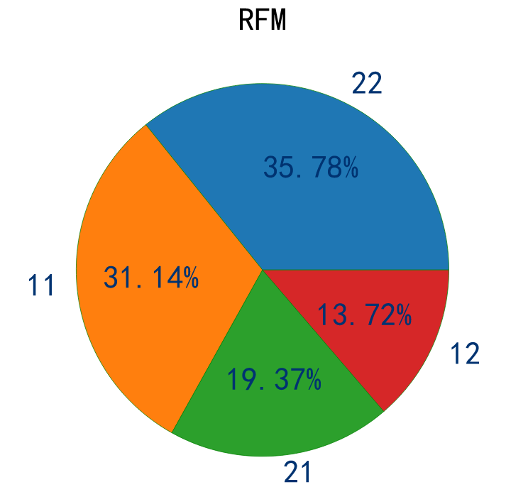
Through RF user value analysis, for 22 users, it is a key user and needs attention; For those with high loyalty and insufficient purchase frequency, users can increase their purchase frequency by means of activity coupons and so on; For 12 such users with low loyalty and low consumption frequency, they need to pay attention to their shopping habits, do more push and precision marketing.
rfm.groupby(['rfm']).count()
| user_id | recent | freq | recent_value | freq_value | |
|---|---|---|---|---|---|
| rfm | |||||
| 11 | 2767 | 2767 | 2767 | 2767 | 2767 |
| 12 | 1219 | 1219 | 1219 | 1219 | 1219 |
| 21 | 1721 | 1721 | 1721 | 1721 | 1721 |
| 22 | 3179 | 3179 | 3179 | 3179 | 3179 |
rfm_count = rfm['rfm'].value_counts()
plt.figure(figsize=(8,8))
plt.pie(rfm_count.values,labels=rfm_count.index,autopct='%.2f%%',
       wedgeprops={'linewidth':0.5,'edgecolor':'green'},
       textprops={'fontsize':30,'color':'#003371'}
       )
plt.title('RFM',size=30)
plt.show()