catalogue

1, Introduction

2, Color recognition principle

3, Functional module design

4, Coverage calculation process

5, Software implementation effect

1, Introduction

With the continuous strengthening of the national awareness of ecological and environmental protection, the balance of grassland grass and livestock has been paid more and more attention. The balance of grassland grass and livestock involves "four degrees and one quantity", and this paper mainly studies "coverage". Vegetation coverage refers to the percentage of the vertical projection area of vegetation (including leaves, stems and branches) on the ground in the total area of the statistical area. As an important parameter reflecting surface information, vegetation coverage has always been one of the important research topics in the field of remote sensing. Generally, the measurement methods of vegetation coverage include surface measurement and remote sensing monitoring. In this paper, the color of the picture is recognized, and the vegetation coverage is obtained according to the proportion of vegetation in the total area of the picture.

2, Color recognition principle

(1) Using the cvtColor function interface of OpenCV, the picture format can be converted to HSV format. The green HSV value is H between 35 and 77, S between 43 and 255, and V between 46 and 255;

The green HSV value range is as follows:

	black	ash	white	red	orange	yellow	green	young	blue
Hmin	0	0	0	156	11	26	35	78	100
hmax	180	180	180	180	25	34	77	99	124
smin	0	0	0	43	43	43	43	43	43
smax	255	43	30	255	255	255	255	255	255
Vmin	0	46	221	46	46	46	46	46	46
Vmax	46	220	255	255	255	255	255	255	255

(2) Then, using color recognition, the vegetation coverage is calculated according to the proportion of green area to the total area of the picture;

Read the pictures in the local folder, convert the format of the pictures into the easy to read pixel composition format, then divide the pictures into regions, filter out the effective areas covered by green, then measure the area covered by green area in the total area of the pictures, and finally calculate the percentage of green area.

3, Functional module design

 

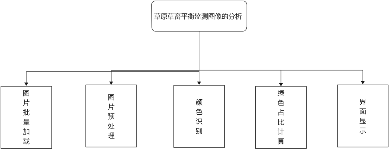
1. Batch loading of pictures: read the local folder and load the pictures saved in the folder

2. Image preprocessing: scaling of images

3. Color recognition: for a specific color, green is recognized

4. Green proportion calculation: the proportion can be calculated according to the selected pictures

5. Display interface: pictures, test results

4, Coverage calculation process

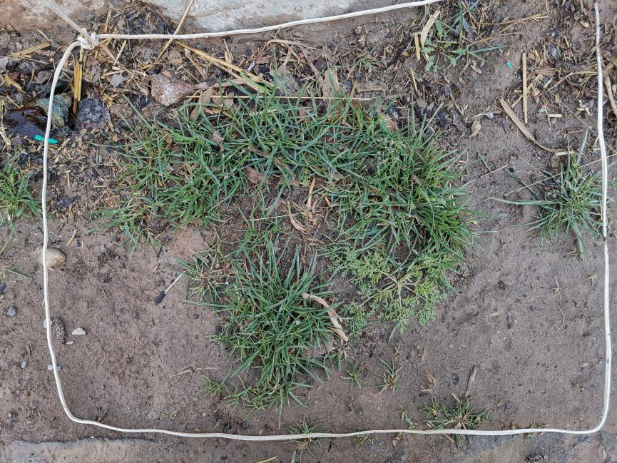
1. Read a picture

Img = cv2.imread(path)  # Read in an image

2. Format the picture

 HSV = cv2.cvtColor(Img, cv2.COLOR_BGR2HSV) # Picture format conversion

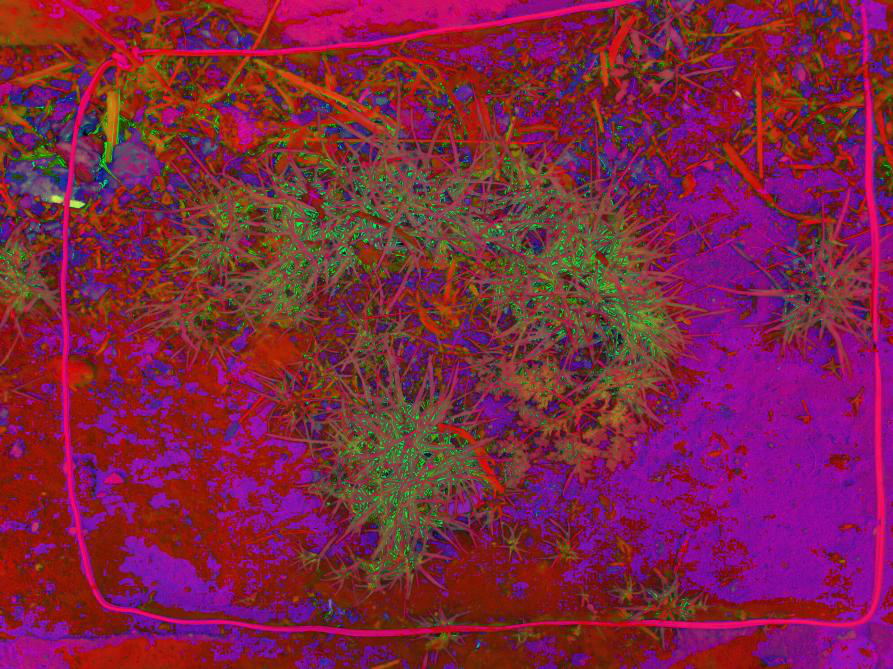
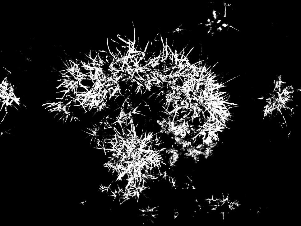
3. Turn the area in the color range of the picture into white and the other areas into black

 self.Lower = np.array([35, 43, 46])  # Lower limit of color to be recognized

 self.Upper = np.array([77, 255, 255])  # The upper limit of the color to be recognized

 mask = cv2.inRange(HSV, self.Lower, self.Upper)

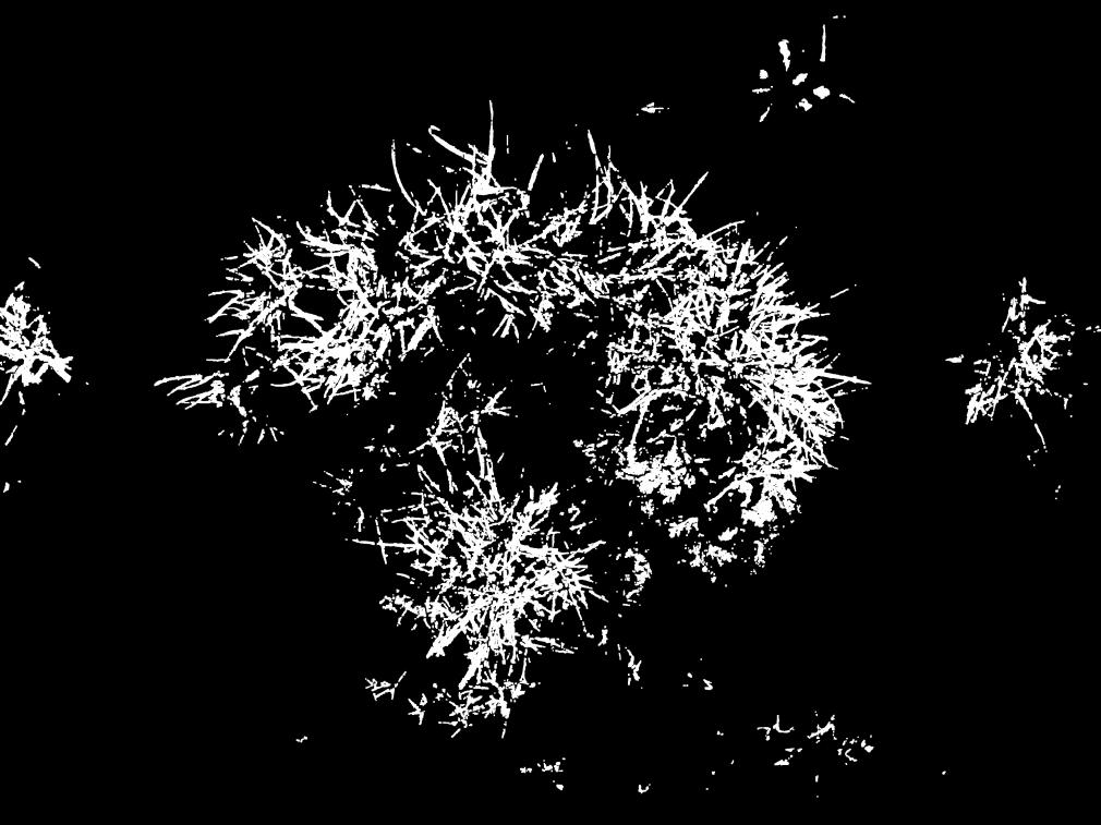
4. Filter pictures

# The following four lines are filter operations

  # The erode() function can operate the input image with a specific structural element, which determines the shape of the neighborhood in the operation process,

  # The pixel value of each point will be replaced with the minimum value on the corresponding neighborhood:

  erosion = cv2.erode(mask, self.kernel_3, iterations=1)

  erosion = cv2.erode(erosion, self.kernel_3, iterations=1)

  # The dilate() function can operate the input image with a specific structural element, which determines the shape of the neighborhood during the operation,

  # The pixel value of each point will be replaced with the maximum value on the corresponding neighborhood:

  dilation = cv2.dilate(erosion, self.kernel_3, iterations=1)

  dilation = cv2.dilate(dilation, self.kernel_3, iterations=1)

 

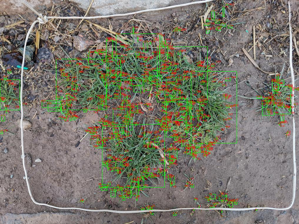
5. Detect the contour of the object, read all the contours, and draw a rectangular mark on the image

 # The outline is found in binary. The outline is arranged from small to large in area

 binary, contours, hierarchy = cv2.findContours(binary, cv2.RETR_EXTERNAL, cv2.CHAIN_APPROX_SIMPLE)

p = 0

green_area = 0

for i in contours:  # Read all contours

 x, y, w, h = cv2.boundingRect(i)  # Decompose the contour into the coordinates of the upper left corner and the width and height of the recognition object

green_area += w * h

# Draw a rectangle on the image (picture, upper left corner coordinate, lower right corner coordinate, color, line width)

cv2.rectangle(Img, (x, y), (x + w, y + h), (0, 255,), 3)

# Mark the identified object

 font = cv2.FONT_HERSHEY_SIMPLEX

cv2.putText(Img, str(p),(x - 10, y + 10), font, 1,(0,0,255), 2)  # Plus or minus 10 is to adjust the character position

 p += 1

6. Calculation method of green proportion

First calculate the total size of the picture

total_area = Img.shape[0]*Img.shape[1]  # total area

Then calculate all green areas and sum them

for i in contours:  # Traverse all contours

x, y, w, h = cv2.boundingRect(i)  # Decompose the contour into the coordinates of the upper left corner and the width and height of the recognition object

green_area += w * h

 p += 1

 print('green The number of squares is', p, 'individual')  # Number of terminal output targets

Final calculated percentage

 percent = (green_area / total_area)*100

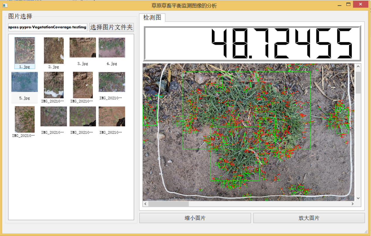
5, Software implementation effect

Enter the interface and select a folder with pictures

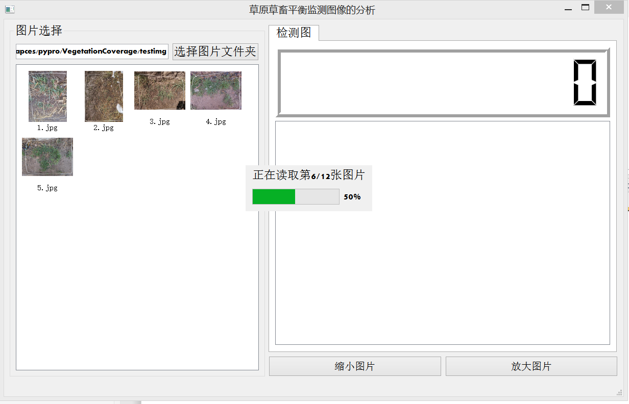
After loading, click the picture on the left to display the test result, which supports the zoom in and zoom out of the picture

Grassland grass and livestock balance monitoring image analysis system Python document resources CSDN Download