1 background
1.1 overview of k-nearest neighbor algorithm
(1) Introduction of k-nearest neighbor algorithm
k-nearest neighbor algorithm is a very effective and easy to master machine learning algorithm. In short, it is an algorithm to classify data by measuring the distance between different eigenvalues.
(2) Working principle of k-nearest neighbor algorithm
Given a set of samples, it is called training set here, and each data in the sample contains labels. For a newly input data without labels, by calculating the distance between the new data and each sample, select the first k, usually K less than 20, and take the label that appears the most frequently among the labels of the latest data in the K series as the newly added data label.
(3) Case of k-nearest neighbor algorithm
At present, the number of kissing and fighting scenes in 6 films is counted. Suppose there is an unseen film, how to determine whether it is a love film or an action film?
| Movie title | Fighting lens | Kissing lens | Film type |
| California Man | 3 | 104 | affectional film |
| He's Not Really into Dudes | 2 | 100 | affectional film |
| Beautiful Woman | 1 | 81 | affectional film |
| Kevin Longblade | 101 | 10 | action movie |
| Robo Slayer 3000 | 99 | 5 | action movie |
| Amped II | 98 | 2 | action movie |
| ? | 18 | 90 | unknown |
According to the principle of knn algorithm, we can find the distance between the unknown movie and each movie (European distance is used here)
Take California Man as an example
>>>((3-18)**2+(104-90)**2)**(1/2)
20.518284528683193
| Movie title | Distance from unknown i movies |
| California Man | 20.5 |
| He's Not Really into Dudes | 18.7 |
| Beautiful Woman | 19.2 |
| Kevin Longblade | 115.3 |
| Robo Slayer 3000 | 117.4 |
| Amped II | 118.9 |
Therefore, we can find the first k nearest films in the sample. Assuming k=3, the first three films are all romantic films. Therefore, we determine that the unknown film belongs to romantic films.
one point two Implementation of k-nearest neighbor algorithm with python code
(1) Calculates the distance between each point in a known category dataset and the current point
(2) Sort by increasing distance
(3) Select the k points with the smallest distance from the current point
(4) Determine the frequency of occurrence of the category where the first k points are located
(5) The category with the highest frequency of the first k points is returned as the prediction classification of the current point
import numpy as np
import operator

def classify0(inX, dataSet, labels, k):
    dataSetSize = dataSet.shape[0]
    diffMat = np.tile(inX, (dataSetSize,1)) - dataSet
    sqDiffMat = diffMat**2
    sqDistances = sqDiffMat.sum(axis=1)
    distances = sqDistances**0.5
    sortedDistIndicies = distances.argsort()
    classCount={}
    for i in range(k):
        voteIlabel = labels[sortedDistIndicies[i]]
        classCount[voteIlabel] = classCount.get(voteIlabel,0) + 1
    sortedClassCount = sorted(classCount.items(), key=operator.itemgetter(1), reverse=True)
    return sortedClassCount[0][0]
(6) Case
>>>group = np.array([[1, 1.1],
...                 [1, 1],
...                 [0, 0],
...                 [0, 0.1]])
>>>labels = ['A', 'A', 'B', 'B']
>>>classify0([0,0], group, labels, 3)
'B'
one point three How to test classifiers
Normally, in order to test the classification effect given by the classifier, we usually calculate the error rate of the classifier to judge the effect of the classifier. That is, divide the number of classification errors by the total number of classification. The error rate of the perfect classifier is 0, while the error rate of the worst classifier is 1.
2 use kNN algorithm to improve the matching effect of dating websites
2.1 case introduction
When my friend Helen uses dating software to find a date, although the website will recommend different candidates, she doesn't like everyone. Specifically, she can be divided into the following three categories: people she doesn't like, people with ordinary charm and people with great charm. Despite the above rules, Helen still can't classify the people recommended by the website into the appropriate category, so Helen I hope our classification software can better help her assign the matched objects to the exact classification.
2.2 data preparation
There are two channels for downloading data sets:
Code of python2 version downloaded by machine learning practice official
github download Python 3 version code for 202xxx
The data is stored in datingTestSet2.txt. Each sample occupies one row, a total of 1000 rows of data, mainly including the following three features:
Frequent flyer miles earned per year, percentage of time spent playing video games, and litres of ice cream consumed per week
Before the data is input into the classifier, it is necessary to convert the data into a style that can be recognized by the classifier
def file2matrix(filename):
    fr = open(filename)
    numberOfLines = len(fr.readlines())         #get the number of lines in the file
    returnMat = np.zeros((numberOfLines,3))        #prepare matrix to return
    classLabelVector = []                       #prepare labels return
    fr = open(filename)
    index = 0
    for line in fr.readlines():
        line = line.strip()
        listFromLine = line.split('\t')
        returnMat[index,:] = listFromLine[0:3]
        classLabelVector.append(int(listFromLine[-1]))
        index += 1
    return returnMat,classLabelVector
The characteristic data (datingDataMat) read using file2matix is as follows
array([[4.0920000e+04, 8.3269760e+00, 9.5395200e-01],
        [1.4488000e+04, 7.1534690e+00, 1.6739040e+00],
        [2.6052000e+04, 1.4418710e+00, 8.0512400e-01],
        ...,
        [2.6575000e+04, 1.0650102e+01, 8.6662700e-01],
        [4.8111000e+04, 9.1345280e+00, 7.2804500e-01],
        [4.3757000e+04, 7.8826010e+00, 1.3324460e+00]]
The datainglabels are as follows
[3,2,1,1,1,1,3,3,...,3,3,3]
two point three Data analysis: creating scatter charts using Matplotlib
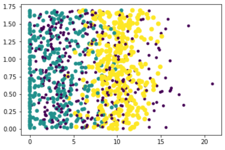
(1) Correlation between percentage of time spent playing video games and litres of ice cream consumed per week
import matplotlib
import matplotlib.pyplot as plt
fig = plt.figure()
ax = fig.add_subplot(111)
ax.scatter(datingDataMat[:,0], datingDataMat[:,1], 15.0*np.array(datingDLabels), 15.0*np.array(datingDLabels))
plt.show()
Where, y-axis is the liters of ice cream consumed per week, and x-axis is the percentage of time spent playing video games
Purple means dislike, green means general charm, and yellow means great charm
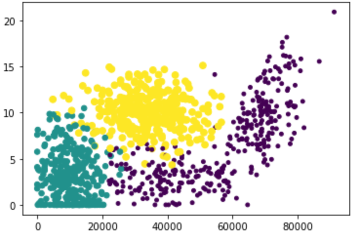
(2) Relationship between frequent flyer mileage and percentage of time spent playing video games
import matplotlib
import matplotlib.pyplot as plt
fig = plt.figure()
ax = fig.add_subplot(111)
ax.scatter(datingDataMat[:,0], datingDataMat[:,1], 15.0*np.array(datingDLabels), 15.0*np.array(datingDLabels))
plt.show()
Where, y-axis is the percentage of time spent playing video games, and x-axis is the frequent flyer mileage
Purple means dislike, green means general charm, and yellow means great charm
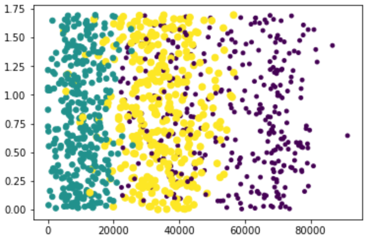
(3) Relationship between frequent flyer mileage and ice cream litres consumed per week
import matplotlib
import matplotlib.pyplot as plt
fig = plt.figure()
ax = fig.add_subplot(111)
ax.scatter(datingDataMat[:,0], datingDataMat[:,2], 15.0*np.array(datingDLabels), 15.0*np.array(datingDLabels))
plt.show()
Where, y-axis is the litres of ice cream consumed per week, and x-axis is the frequent flyer mileage
Purple means dislike, green means general charm, and yellow means great charm
two point four Data preparation: normalized value
When calculating the distance between samples through European distance, the number of frequent flyer miles is huge, and the weight that will affect the results will be large, and far greater than the other two features. However, as one of the three equal weights, frequent flyer miles should not affect the results so seriously, as shown in the following examples
((0-67)**2+(20000-32000)**2+(1.1-0.1)**2)**1/2
| Percentage of time spent playing video games | Frequent flyer mileage | Litres of ice cream consumed per week | Sample classification | |
| 1 | 0.8 | 400 | 0.5 | 1 |
| 2 | 12 | 134000 | 0.9 | 3 |
| 3 | 0 | 20000 | 1.1 | 2 |
| 4 | 67 | 32000 | 0.1 | 2 |
Usually, when dealing with features with different value ranges, we often use normalization to map the eigenvalues to 0-1 or - 1 to 1, and normalize the features by (all values in the column - minimum value in the column) / (maximum value in the column - minimum value in the column)
def autoNorm(dataSet):
    minVals = dataSet.min(0)
    maxVals = dataSet.max(0)
    ranges = maxVals - minVals
    normDataSet = np.zeros(np.shape(dataSet))
    m = dataSet.shape[0]
    normDataSet = dataSet - np.tile(minVals, (m,1))
    normDataSet = normDataSet/np.tile(ranges, (m,1))   #element wise divide
    return normDataSet, ranges, minVals
two point five Test algorithm: verify the classifier as a complete program
Evaluating the accuracy is a very important step in machine learning algorithms. Usually, we only use 90% of the training samples to train the classifier, and the remaining 10% to test the accuracy of the classifier. In order not to affect the randomness of the data, we need to randomly select 10% of the data.
(1) Use the file2matrix function to import data samples
(2) Normalize the data using autoNorm
(3) Use classify0 to train 90% of the data and test 10% of the data
(4) Error rate in output test set
def datingClassTest():
    hoRatio = 0.50      #hold out 10%
    datingDataMat,datingLabels = file2matrix('datingTestSet2.txt')       #load data setfrom file
    normMat, ranges, minVals = autoNorm(datingDataMat)
    m = normMat.shape[0]
    numTestVecs = int(m*hoRatio)
    errorCount = 0.0
    for i in range(numTestVecs):
        classifierResult = classify0(normMat[i,:],normMat[numTestVecs:m,:],datingLabels[numTestVecs:m],3)
        print ("the classifier came back with: %d, the real answer is: %d" % (classifierResult, datingLabels[i]))
        if (classifierResult != datingLabels[i]): errorCount += 1.0
    print ("the total error rate is: %f" % (errorCount/float(numTestVecs)))
    print (errorCount)
Finally, the error rate of the appointment dataset processed by the classifier is 2.4%, which is a very good result. Similarly, we can change the value of hoRatio and k to detect whether the error rate increases with the change of variables
two point five Using algorithms: building a complete and usable system
Through the above learning, we try to develop a program for Helen. By finding someone's information on the dating website and inputting it into the program, the program will give Helen's prediction of her liking for each other: dislike, general charm and great charm
import numpy as np
import operator

def file2matrix(filename):
    fr = open(filename)
    numberOfLines = len(fr.readlines())         #get the number of lines in the file
    returnMat = np.zeros((numberOfLines,3))        #prepare matrix to return
    classLabelVector = []                       #prepare labels return
    fr = open(filename)
    index = 0
    for line in fr.readlines():
        line = line.strip()
        listFromLine = line.split('\t')
        returnMat[index,:] = listFromLine[0:3]
        classLabelVector.append(int(listFromLine[-1]))
        index += 1
    return returnMat,classLabelVector

def autoNorm(dataSet):
    minVals = dataSet.min(0)
    maxVals = dataSet.max(0)
    ranges = maxVals - minVals
    normDataSet = np.zeros(np.shape(dataSet))
    m = dataSet.shape[0]
    normDataSet = dataSet - np.tile(minVals, (m,1))
    normDataSet = normDataSet/np.tile(ranges, (m,1))   #element wise divide
    return normDataSet, ranges, minVals

def classify0(inX, dataSet, labels, k):
    dataSetSize = dataSet.shape[0]
    diffMat = np.tile(inX, (dataSetSize,1)) - dataSet
    sqDiffMat = diffMat**2
    sqDistances = sqDiffMat.sum(axis=1)
    distances = sqDistances**0.5
    sortedDistIndicies = distances.argsort()
    classCount={}
    for i in range(k):
        voteIlabel = labels[sortedDistIndicies[i]]
        classCount[voteIlabel] = classCount.get(voteIlabel,0) + 1
    sortedClassCount = sorted(classCount.items(), key=operator.itemgetter(1), reverse=True)
    return sortedClassCount[0][0]

def classifyPerson():
    resultList = ["not at all", "in small doses", "in large doses"]
    percentTats = float(input("percentage of time spent playing video games?"))
    ffMiles = float(input("ferquent fiter miles earned per year?"))
    iceCream = float(input("liters of ice ice crean consumed per year?"))
    datingDataMat,datingLabels = file2matrix('knn/datingTestSet2.txt')       #load data setfrom file
    normMat, ranges, minVals = autoNorm(datingDataMat)
    inArr = np.array([percentTats, ffMiles, iceCream])


    classifierResult = classify0((inArr-minVals)/ranges, normMat, datingLabels,3)
    print ("You will probably like this person:", resultList[classifierResult-1])

if __name__ == "__main__":
    classifyPerson()#10    10000    0.5
Enter test data:
percentage of time spent playing video games?10
ferquent fiter miles earned per year?10000
liters of ice ice crean consumed per year?0.5
You will probably like this person: not at all
3 use kNN algorithm to make handwriting recognition system
3.1 case introduction
Taking the classification of numbers 0-9 as an example, the following case briefly describes how to use k-nearest neighbor algorithm to recognize handwritten numbers.
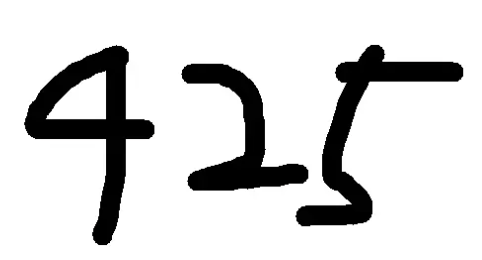
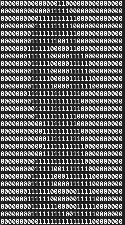
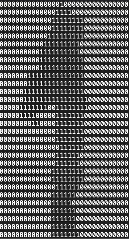
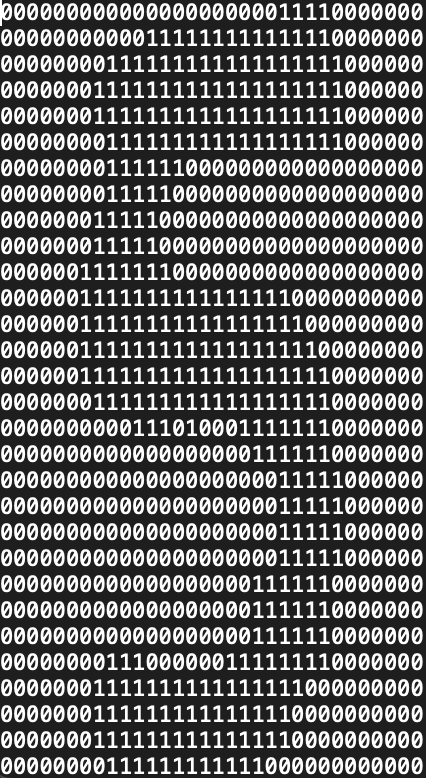
Generally, the handwritten input numbers are in picture format. We need to convert the picture into structured data that can be recognized by knn algorithm. In short, we need to read the pixels in the picture. The pixel values are usually between 0-255, 0 is black and 255 is white. Therefore, the pixels with values greater than 250 can be marked as 1 and the rest as 0. The handwritten numeral 1 can be represented by the following data set:
| 1 | 1 | 1 | 1 | 1 | 1 | 1 | 1 | 1 | 1 |
| 1 | 1 | 1 | 1 | 0 | 0 | 0 | 1 | 1 | 1 |
| 1 | 1 | 1 | 1 | 0 | 0 | 0 | 1 | 1 | 1 |
| 1 | 1 | 1 | 1 | 0 | 0 | 1 | 1 | 1 | 1 |
| 1 | 1 | 1 | 1 | 0 | 0 | 1 | 1 | 1 | 1 |
| 1 | 1 | 1 | 1 | 0 | 0 | 1 | 1 | 1 | 1 |
| 1 | 1 | 1 | 1 | 0 | 0 | 1 | 1 | 1 | 1 |
| 1 | 1 | 1 | 1 | 0 | 0 | 1 | 1 | 1 | 1 |
| 1 | 1 | 1 | 0 | 0 | 0 | 0 | 1 | 1 | 1 |
| 1 | 1 | 1 | 1 | 1 | 1 | 1 | 1 | 1 | 1 |
three point two Data preparation: converting images into test vectors
There are two channels for downloading data sets:
Code of python2 version downloaded by machine learning practice official
github download Python 3 version code for 202xxx
The dataset is stored in digits.zip, where 1 represents the handwritten area and 0 represents the blank area
(big guys, Happy Mid Autumn Festival!!!)
The data is read through the img2vector function and an array is returned
def img2vector(filename):
    returnVect = np.zeros((1,1024))
    fr = open(filename)
    for i in range(32):
        lineStr = fr.readline()
        for j in range(32):
            returnVect[0,32*i+j] = int(lineStr[j])
    return returnVect
3.3 test the algorithm and use kNN to recognize handwritten digits
(1) Use listdir to read all files in the trainingDigits directory as training data
(2) Use listdir to read all files in the testDigits directory as test data
(3) The training data and test data are fed into the knn algorithm
def handwritingClassTest():
    hwLabels = []
    trainingFileList = listdir('trainingDigits')           #load the training set
    m = len(trainingFileList)
    trainingMat = np.zeros((m,1024))
    for i in range(m):
        fileNameStr = trainingFileList[i]
        fileStr = fileNameStr.split('.')[0]     #take off .txt
        classNumStr = int(fileStr.split('_')[0])
        hwLabels.append(classNumStr)
        trainingMat[i,:] = img2vector('trainingDigits/%s' % fileNameStr)
    testFileList = listdir('testDigits')        #iterate through the test set
    errorCount = 0.0
    mTest = len(testFileList)
    for i in range(mTest):
        fileNameStr = testFileList[i]
        fileStr = fileNameStr.split('.')[0]     #take off .txt
        classNumStr = int(fileStr.split('_')[0])
        vectorUnderTest = img2vector('testDigits/%s' % fileNameStr)
        classifierResult = classify0(vectorUnderTest, trainingMat, hwLabels, 3)
        print ("the classifier came back with: %d, the real answer is: %d"% (classifierResult, classNumStr))
        if (classifierResult != classNumStr): errorCount += 1.0
    print ("\nthe total number of errors is: %d" % errorCount)
    print ("\nthe total error rate is: %f" % (errorCount/float(mTest)))
Output the training results, the error rate is 1.1628%, and the error rate will change by changing the k value and training samples.
the classifier came back with: 7, the real answer is: 7
the classifier came back with: 7, the real answer is: 7
the classifier came back with: 9, the real answer is: 9
the classifier came back with: 0, the real answer is: 0
the classifier came back with: 0, the real answer is: 0
the classifier came back with: 4, the real answer is: 4
the classifier came back with: 9, the real answer is: 9
the classifier came back with: 7, the real answer is: 7
the classifier came back with: 7, the real answer is: 7
the classifier came back with: 1, the real answer is: 1
the classifier came back with: 5, the real answer is: 5
the classifier came back with: 4, the real answer is: 4
the classifier came back with: 3, the real answer is: 3
the classifier came back with: 3, the real answer is: 3

the total number of errors is: 11

the total error rate is: 0.011628
4 Summary
4.1 advantages and disadvantages of k-nearest neighbor algorithm
(1) Advantages: high precision, insensitive to outliers, no data input assumption
(2) Disadvantages: high computational complexity and space complexity
Applicable data range: numerical type and nominal type
four point two General flow of k-nearest neighbor algorithm
(1) Collect data: any method can be used
(2) Prepare data: the value required for distance calculation, preferably in a structured data format
(3) Analyze data L: any method can be used
(4) Training algorithm: this step is not suitable for k-nearest neighbor algorithm
(5) Test algorithm: calculate error rate
(6) Using the algorithm: first, input the sample data and structured output results, then run the k-nearest neighbor algorithm to determine which classification the input data belongs to respectively, and finally perform subsequent processing on the calculated classification.
four point three Problems needing attention in the use of k-nearest neighbor algorithm
(1) When the dimensions of data features are not unified, the data needs to be normalized, otherwise there will be a problem that large numbers eat decimals
(2) The distance between data is usually calculated by European distance
(3) The selection of K value in kNN algorithm will have a great impact on the results. Generally, K value is less than the square root of training sample data
(4) The cross validation method is usually used to select the optimal K value
5 Reference
Machine learning practice