After learning the third chapter of Robotics, Vision and Control, I found that the book has supporting videos. It's hard to read the second chapter. I have a hard understanding of many places. Now I'm going to have a good look at the videos and take notes as a supplement.

References for this series:

1. <Robotics, Vision and Control>

2. Open class at station B:

   1. Open course of robotics, Taiwan Jiaotong University
   2. Peter Corke companion video

3. Lao Huang's course explanation and PPT of fundamentals of robot technology

4. N many blogs about big guys in Robotics

   Recommend a blog: Summary of MATLAB RTB common formulas (III) , I corrected some of my notes with reference to it.

00 overview

In the first part, we learned the description of object pose in two-dimensional and three-dimensional space. In this part, we mainly study the description of object pose over time, so as to pave the way for the chassis, navigation and positioning of the rear robot.

01 track

Path: a figure from initial pose - > final pose.

Track: path + specific time attribute; The important feature of trajectory is smoothness, and the position and posture need to change smoothly with time.

01-1 smooth one-dimensional trajectory

One dimension represents a straight line. We can use a common real function to express the change law of pose with time. Let's take quintic polynomial function as an example:

Its trajectory equation, derivative and second derivative are as follows:

Given such an equation, we can determine the boundary of position, velocity and acceleration. If we take t=0 and t=T into the above three formulas, we can get a matrix.

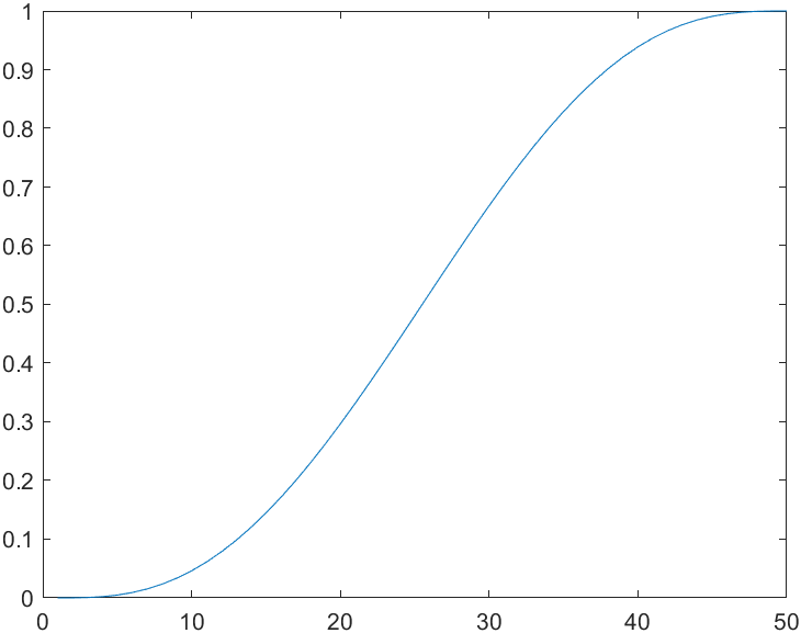
s = tpoly(0, 1, 50);
%Generate a quintic polynomial trajectory, 0~1，50 steps
%Output:
s = 50×1    
    0.0021
    0.0048
    0.0091
    0.0152
    0.0233
    0.0336
    0.0461
    0.0611
    0.0785
    0.0982
    ...
plot(s)
% Draw the trajectory curve as follows:
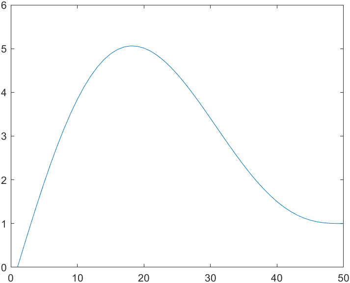
[s, sd, sdd] = tpoly(0,1,50);
% Output speed and acceleration
% If you want to output speed and acceleration
subplot(3,2,1);plot(s1);grid on;xlabel('time');ylabel('s');
subplot(3,2,3);plot(sd1);grid on;xlabel('time');ylabel('sd');
subplot(3,2,5);plot(sdd1);grid on;xlabel('time');ylabel('sdd');

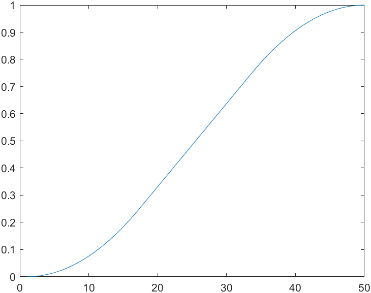
% Set 0~1,50 step,Initial speed 0.5,The final speed is 0
s1 = tpoly(0,1,50,0.5,0);
plot(s1)
% If you want to output speed and acceleration, do the same as above

1. From the perspective of trajectory, this situation will make the motion have a reciprocating phenomenon, that is, some points exceed the end point (one dimension). For example, the peak value in the image is 5, which is beyond the range of 0 ~ 1.

2. In terms of speed, in the first case (taking 0 as the initial speed), the maximum speed will be obtained in 25s (we can draw it with plot). We can use the following code to calculate the average speed:

   mean(sd)/max(sd)
   % Output:
   ans = 0.5231
   % That is, the average speed is 52% of the maximum speed.31%
   

We know that the real robot joint has a rated speed. We generally hope that the robot (joint) will reach the specified position as soon as possible, even if its proportion is as large as possible when the speed is high.

One solution is to use a mixed curve trajectory:

s2 = lspb(0, 1, 50)
% The trajectory consists of a line segment (representing uniform motion) and two parabolas
plot(s2)

It can be predicted that the speed curve of this movement is a trapezoid, so it also becomes a trapezoidal trajectory, which is widely used in the field of industrial motor drive.

Although the velocity of trapezoidal trajectory is smooth, the acceleration is not smooth.

The lspb above is the default speed. We can set the parameters ourselves to give a speed to the straight line segment (of course, the speed value is not arbitrarily selected):

% Let's first return to the straight-line segment velocity of the current graph as a reference
max(sd)
% Output:
ans = 0.0306
% Then set the new parameter 0.025，Infeasible parameters return an error
s2 = lspb(0, 1, 50, 0.025);

01-2 multidimensional trajectory

We need a multi-dimensional vector to describe an object, and most of us need to know that it is a multi-dimensional vector; To describe the motion of an object, we also need to describe the multidimensional smooth motion from the initial pose vector to the final initial pose vector.

It is still very simple to expand the scalar trajectory of 01-1 into multi-dimensional vectors in RTB, that is, use mtraj function.

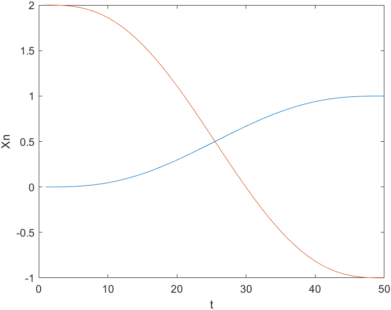
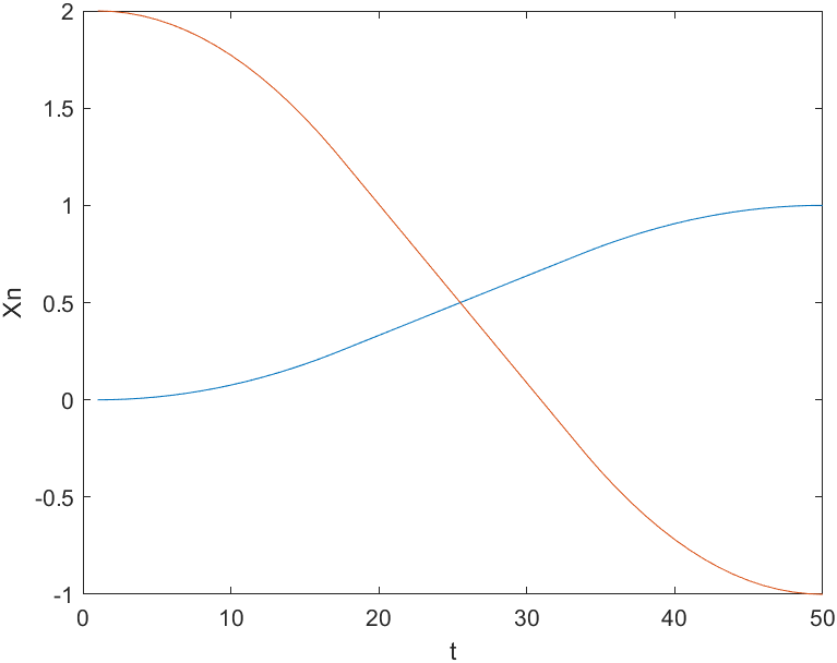
x = mtraj(@tpoly, [0 2], [1 -1], 50);
% %In 50 time steps(0,2)Move to(1,-1)，According to 50×2 The matrix generates a two variable scalar trajectory
% x = mtraj(@lspb, [0 2], [1 -1], 50);
plot(x);
% In fact, it's not standard,The horizontal axis is time and the vertical axis is each dimension x scalar 
xlabel('t')
ylabel('Xn')

% For three-dimensional pose, if it is three variables, the meaning is as follows, and so on
x = mtraj(@tpoly, [0 2 1], [1 -1 0], 50);

If lspb function is used, it is shown in the following figure:

For the pose problem in three-dimensional space, the pose homogeneous matrix T can be transformed into a six-dimensional vector by the following method:

x = [transl(T); tr2rpy(T)'];
% transl Realize translation operation tr2rpy Is pose homogeneous matrix T->Cardan angles (Describe rotation angle)

Then the corresponding trajectory is generated. However, there are some limitations on the triangulation interpolation to describe the attitude. I'll talk about that later.

01-3 multi segment trajectory

Robot applications often need to move smoothly along a path and pass through one or more intermediate points without stopping.

We can concretize the problem, that is, we need to let the trajectory pass through N points xn (pose vector) that can determine this path, that is, it is divided into N-1 motion intervals.

The original translation of the following paragraphs is not good. Most online bloggers only make records, but in fact, it does not delay the students with engineering foundation to understand the meaning. I understand and sort out as follows:

one-dimensional

Put the original picture first (with e-book hee hee):

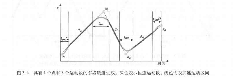
According to the above meaning, for example (as shown in Figure 3.4 of the e-book above), we consider a one-dimensional case. After all, from 01-2, we can see that multi dimensions are only a combination of one dimensions, and each dimension is a one-dimensional motion.

This case requires us to arrive at X4 from X1. The path decision points (intermediate points) we selected are X1, X2, X3 and X4. Note that the selection here does not mean that we must completely pass through these points. We need to integrate all requirements and plan a reasonable scheme. Attach one-dimensional picture:

At the simplest, we will connect X1-X2-X3-X4 in turn, but obviously our speed will become discontinuous: because X2 is even on the right side of X4, if we outline the broken line content in Figure 3.4 of the book, there will be a sudden change in speed.

In order to achieve speed continuity, we need to abandon some predetermined middle point positions (actually well understood from the perspective of calculation method / numerical analysis) and adopt the method of straight line and curve fitting, such as the combination of curves and straight lines in the book. In this way, the picture in the book will be well understood:

1. Accelerate from X1 according to the required acceleration (not necessarily constant) to a uniform speed;
2. Note that this uniform speed can be set as required;
3. Moving at a uniform speed to an appropriate time, that is, the time when tacc/2 time is required according to the predetermined straight line, that is, the end time of the first straight line in the figure;
4. The process of starting deceleration and then reverse acceleration, which corresponds to the tacc time in the figure;
5. Repeat the above similar process.

We can also calculate the average acceleration of the fourth step

If the maximum acceleration of the axis corresponding to this dimension is known, the minimum tacc can be calculated.

Multidimensional

Let's learn more about multidimensional:

As mentioned above, multidimensional is just a combination of one dimension. The most important problem to consider when combining one dimension is that we need to make the points in different dimensions reach the next target point Xk at the same time.

The solution is to consider the simple short board effect: we consider the movement of the dimension that takes the longest time from Xk to Xk+1. Calculate the specific time according to the rated speed and the distance of this dimension, and then further determine the actual required speed of each dimension.

Matlab implementation

% mstraj()A multi segment and multi axis trajectory can be generated according to the intermediate point matrix
via = [4,1; 4,4; 5,2; 2,5];
q = mstraj(via, [2, 1], [], [4, 1], 0.05, 0);
% Parameters: via Intermediate point, maximum velocity vector, time vector of each section, starting point, sampling time interval and acceleration time will output a position matrix divided by sampling points
plot(q)

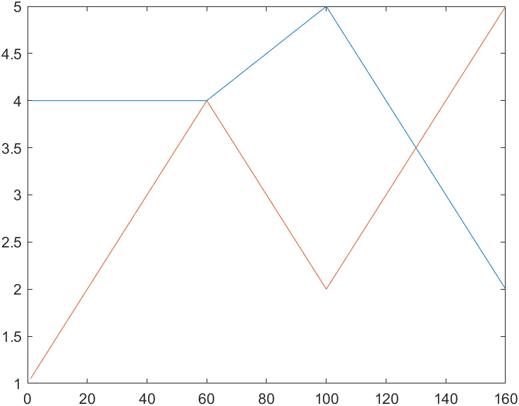
It can be seen that we have not set the acceleration time in the above code. If we set the acceleration time tacc, the above polyline will become more rounded.

% mstraj()A multi segment and multi axis trajectory can be generated according to the intermediate point matrix, which should be consistent with the generation of quintic polynomial mtraj Distinguish
q = mstraj(via, [2, 1], [], [4, 1], 0.05, );

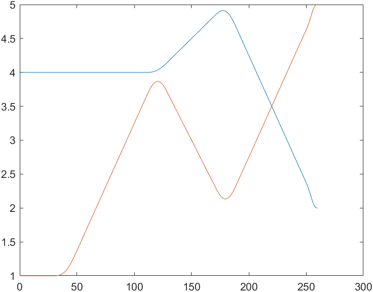
It is worth noting that this mstraj() parameter is very rich. For example, the speed of the starting point and the ending point can be passed in. tacc can be a vector to set the time of each speed change. Mstraj interpolates the pose represented by the vector. Our example is the vector in Cartesian coordinate system, which can also be applied to the vector of three vector representation.

However, for attitude rotation, there will be a better interpolation method:

01-4 3D spatial attitude interpolation

Use superscripts and subscripts in typera:

1. Superscript: content
2. Subscript: content

In robotics, we often need to interpolate the pose. For example, for the end effector, from the pose ξ 0 changed to ξ 1, we need a continuous function ξ (s) = σ ( ξ 0 ξ 1, s) (s∈[0, 1])； The boundary condition of this function is easy to know as σ ( ξ 0 ξ 1, 0) = ξ 0 σ ( ξ 0 ξ 1, 1) = ξ 1.

It must be emphasized here that this function must pass through a series of intermediate poses smoothly, and how to realize it depends on ξ The representation of (as mentioned in the previous part).

Review interpolation:

The continuous function is interpolated on the basis of discrete data to make this continuous curve pass through all given discrete data points.

If ξ The representation of is orthogonal rotation matrix. If simple linear interpolation is used, the interpolated matrix is not orthogonal.

Review matrix Orthogonality:

The orthogonal matrix satisfies that the norm of column vector 2 is 1, and the & & column vectors are orthogonal.

The trigonometric representation enables linear interpolation:

However, according to the content of the previous part, there are singularities in the triangulation representation.

The interpolation method of unit quaternion is similar to that of three angles. See matlab representation.

Quaternion interpolation is realized by using spherical linear interpolation (slerp), in which the unit quaternion moves along a large circle path on a four-dimensional hypersphere and turns around a fixed axis in three-dimensional space.

matlab implementation

%%Trigonometric representation
% Two postures are defined: the initial state and the final state
R0=rotz(-30/pi*180)*roty(30/pi*180);
R1=rotz(30/pi*180)*roty(30/pi*180);
%
% Get equivalent roll-pitch-Yaw angle
rpy0 = tr2rpy(R0);
rpy1 = tr2rpy(R1);
% Generate a track between them in 50 time steps
rpy = mtraj(@tpoly,rpy0,rpy1,50);
tranimate(rpy2tr(rpy));
view([-48.02 30.83]);% Adjust the angle of view to see more clearly
% The moving picture will not be saved at present. The following is the effect picture:

%%Unit quaternion indicates:
% We use the position and pose of the above triangulation and convert it to quaternion first
q0 = UnitQuaternion(R0);
q1 = UnitQuaternion(R1);
% Interpolate them
q = interp(q0, q1,[0:49]'/49);
% Check the interpolation
about(q)
% Animation:
tranimate(q.T)
% The renderings are as follows:

01-5 Cartesian motion

In this part, we study the interpolation of homogeneous transformation matrix.

This problem comes from the fact that we sometimes have a requirement: to generate a smooth path between two poses in SE(3), this process will involve the changes of position and pose at the same time. In robotics, this is often called Cartesian motion.

Combine matlab with practice to understand:

% Create the start and end pose:
T0 = transl(0.4, 0.2, 0)*trotx(180);
T1 = transl(-0.4, -0.2, 0.3)*troty(90)*trotz(-90);
% Here are the questions from these perspectives:
% trotx These functions have no'deg'All descriptions should be in radian system. This is just to make the rotation more extensive

The toolbox function trinterp provides pose interpolation in the unit distance s ∈ [0,1] along the path. For example: middle pose:

trinterp(T0, T1, 0.5)
% Output is:
ans = 4×4    
         0    1.0000         0         0
         0         0   -1.0000         0
   -1.0000         0         0    0.1500
         0         0         0    1.0000

In the translation part, we use linear interpolation, and in the rotation part, we use quaternion interpolation interp for spherical interpolation.

Fifty step-by-step trajectories between the above two poses can be interpolated as follows:

Ts = trinterp(T0, T1, [0:49]/49);
%Generate a homogeneous transformation matrix for each time step
% The parameters correspond to the starting point respectively/The pose of the end point, the path length that varies linearly from 0 to 1.

about(Ts)
% Output:
Ts [double] : 4x4x50 (6.4 kB)
% This is the homogeneous transformation matrix corresponding to each time step(50 Four×4 matrix)
% We can look at the homogeneous transformation of the first point
Ts(:, :, 1)
% Output:
ans = 4×4    
    1.0000         0         0    0.4000
         0   -1.0000         0    0.2000
         0         0   -1.0000         0
         0         0         0    1.0000
% It can be visually displayed through animation:
tranimate(Ts)
% It will show the coordinate system from pose to pose T1 Translation and rotation pose T2 The change process of.
% The translation part of the track is obtained in the following way:
 P = transl(Ts)
% The Cartesian position coordinates of the output trajectory can be compared with our initial and final positions and postures. Each row corresponds to the position vector on each time step.
P = 50×3    
    0.4000    0.2000         0
    0.3837    0.1918    0.0061
    0.3673    0.1837    0.0122
    0.3510    0.1755    0.0184
    0.3347    0.1673    0.0245
    0.3184    0.1592    0.0306
    0.3020    0.1510    0.0367
    0.2857    0.1429    0.0429
    0.2694    0.1347    0.0490
    0.2531    0.1265    0.0551
    ...

% We can plot the change of position: note the change of position
plot(P)

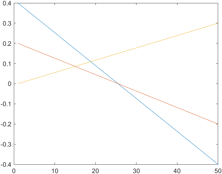
In addition, we can also take a look at the attitude change curve formatted by roll pitch yaw.

rpy = tr2rpy(Ts);
plot(rpy);

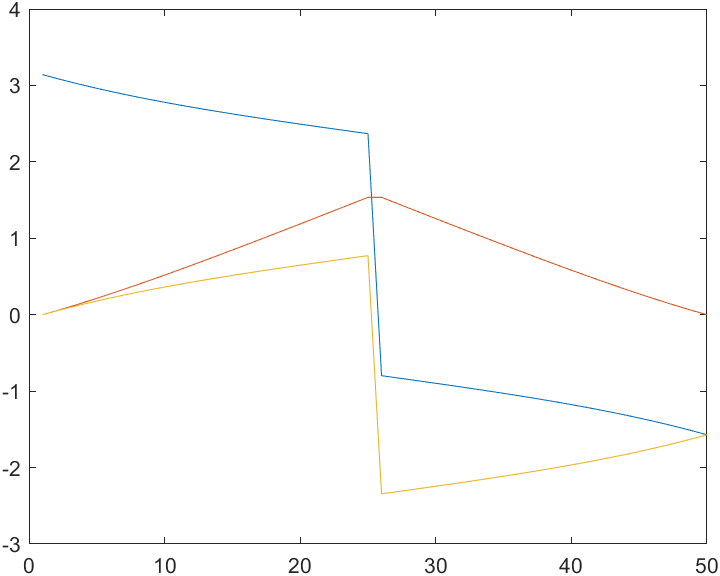
Blue: x roll; Red: y pitch; Yellow: z yaw

It can be seen that the position change is smooth and linear, while the attitude change is neither smooth nor linear. The nonlinearity is due to the nonlinear transformation of the quaternion represented by the angle representation. It's not smooth because of the singularity.

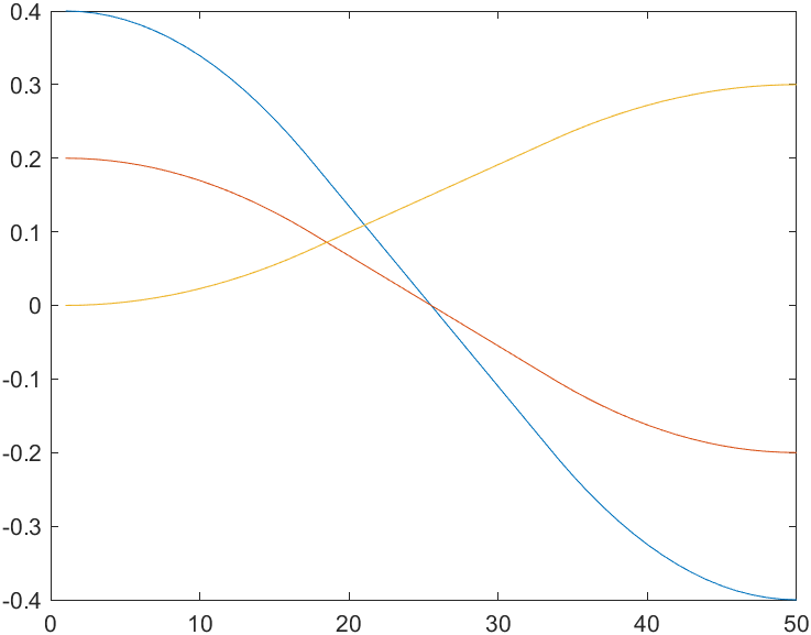
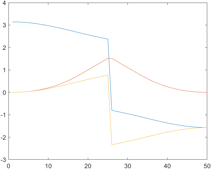
plot is obtained by direct connection. We can use tpoly, lspb or ctraj to smooth the broken lines above. This will not change the trajectory, but it is clear that the speed and acceleration will become much more reasonable.

Ts1 = trinterp(T0, T1, lspb(0,1,50));
P1 = transl(Ts1)
%%
% or Ts = ctraj(T0,T1,50);Beginning and end posture+Step by step quantity
plot(P1)

rpy1 = tr2rpy(Ts1)
plot(rpy1)

02 time varying coordinate system

Above, we study the trajectory of the rotation and translation of the object with time, and below, we study the velocity of the trajectory. The translational speed is easy to say. Let's discuss the rotational speed in detail.

02-1 rotating coordinate system

concept

When we consider the rotation of an object, we usually use the angular velocity vector ω= ( ω x, ω y, ω z) To measure, it may be known from the large object that the angular velocity is an axis, an instantaneous rotation axis, and the vector length represents the rotation rate around the axis.

Think of the rotation around the fixed axis learned in the previous part.

There is a differential expression of time-varying rotation matrix in Mechanics:

R(t) is the standard orthogonal rotation matrix, and the left side is the angular velocity

S( ω) It is a skew symmetric matrix. In three-dimensional case, the specific form is as follows:

matlab implementation

% To get S(ω)matrix
S = skew([1 2 3])
% Output:
S = 3×3    
     0    -3     2
     3     0    -1
    -2     1     0
% vex Can inverse solution S，Get the angular velocity vector
vex(S)
% Output:
ans = 3×1    
     1
     2
     3

further

We can try to understand the left side:

This shows how the orthogonal rotation matrix changes as a function of angular velocity.

02-2 incremental motion

Concept derivation

Following the above derivation, we consider a small rotation R0 - > R1 and get:

δθ=δ t ω Is a three-dimensional vector, the unit is angle, which represents an infinitesimal rotation around the three axes of the world coordinate system xyz.

It is explained below that the multiplication of infinitesimal angle change is exchangeable:

delta1 = rotx(0.001*180/pi)*roty(0.002*180/pi)*rotz(0.003*180/pi)
% Output:
delta1 = 3×3    
    1.0000   -0.0030    0.0020
    0.0030    1.0000   -0.0010
   -0.0020    0.0010    1.0000


%%Change the order:
delta2 = roty(0.002*180/pi)*rotx((0.001*180/pi)*rotz(0.003*180/pi))
% Output:
delta2 = 3×3    
    1.0000   -0.0030    0.0020
    0.0030    1.0000   -0.0010
   -0.0020    0.0010    1.0000
% Using the formula derived above, we can calculate the micro rotation angle 0 corresponding to the matrix.001，0.002，0.003.
vex(delta1 - eye(3,3))'
% Output:
ans = 1×3    
    0.0010    0.0020    0.0030

For two poses with minimal difference ξ 0 ξ 1. A six dimensional vector can be used to represent the difference:

It consists of displacement increment and rotation increment; This difference δ Obviously, space velocity can be used ✖ δ t to calculate the space velocity, which will be studied in the later part of velocity relationship. Now we consider that the pose is expressed in the form of homogeneous transformation matrix:

In the toolbox, tr2delta can be used to solve T.

Let's consider the inverse operation of the previous formula (3.9):

The inverse operation can be solved by delta2tr.

matlab implementation

% Let's determine the beginning and end posture first T0，T1
T0 = transl(1,2,3)*trotx(1*180/pi)*troty(1*180/pi)*trotz(1*180/pi);
T1 = T0 * transl(0.01,0.02,0.03)*trotx(0.001)*troty(0.002)*trotz(0.003)
% Output:
T1 = 4×4    
    0.2889   -0.4547    0.8425    1.0191
    0.8372   -0.3069   -0.4527    1.9887
    0.4644    0.8361    0.2920    3.0301
         0         0         0    1.0000
% (3.10)in▲Is calculated by tr2delta Completed
d = tr2delta(T0, T1);
d' % Just transpose
% Output:
ans = 1×6    
    0.0100    0.0200    0.0300    0.0010    0.0020    0.0030
%% Let's try the inverse transformation and use the homogeneous transformation to act on T0，Take a look at the results and set the final attitude T1 Differences between
delta2tr(d)*T0
ans = 4×4    
    0.2903   -0.4521    0.8434    1.0100
    0.8376   -0.3061   -0.4524    2.0200
    0.4627    0.8378    0.2898    3.0300
         0         0         0    1.0000
% It looks very close. The error comes from that the displacement is not infinitesimal.

Explanation of tr2delta and delta2tr:

tr2delta:

d = tr2delta (T0, T1) converts the homogeneous transformation into differential motion (the difference is a discrete differential), describing the infinitesimal change from attitude t0 to T1. A six dimensional vector d = (dx, dy, dz, dRx, dRy, dRz) will be output, which is the approximate value of the average space velocity multiplied by time.

delta2tr:

Convert differential motion to homogeneous transformation.

02-3 inertial navigation

I think this part can be described separately. After all, inertial navigation can be published separately. This is just for understanding.

Inertial navigation system is a "black box", which is composed of a computer and motion sensor. It inputs its own measured values such as acceleration and angular velocity, and obtains the velocity, direction and position relative to the inertial reference system (universe) through calculation.

No external signal input is required, so it is very suitable for submarines, spacecraft and ballistic missiles.

1. Similar to its principle is the balance sensor in the inner ear.
2. The system integrating various sensors is called inertial measurement unit IMU
3. The design principles of early inertial navigation and modern strapdown inertial navigation are slightly different
4. The basic idea is to obtain the angular velocity and acceleration based on the high working sampling frequency of inertial navigation system, calculate the integral, and obtain the changes of velocity, position and angle to determine the current position and attitude.

03 brief summary | Review

Following the example of the first part, we also need to summarize several macro impressions through the study of this part, so as to facilitate the follow-up in-depth study:

1. Create the trajectory of robot movement. The important feature of the trajectory is smooth, and the time and attitude should change continuously with time.
2. Study on the speed of rotation, we study the time derivative of orthogonal rotation matrix, and we establish the relationship with the angular velocity of mechanics
3. As the application of this part of knowledge, the orthogonal rotation matrix method and quaternion method are used in rotation interpolation and angular velocity integration in inertial navigation. The results of the two methods are equivalent. But the formula of quaternion method is more concise and the calculation is more effective.