Catalogue

 

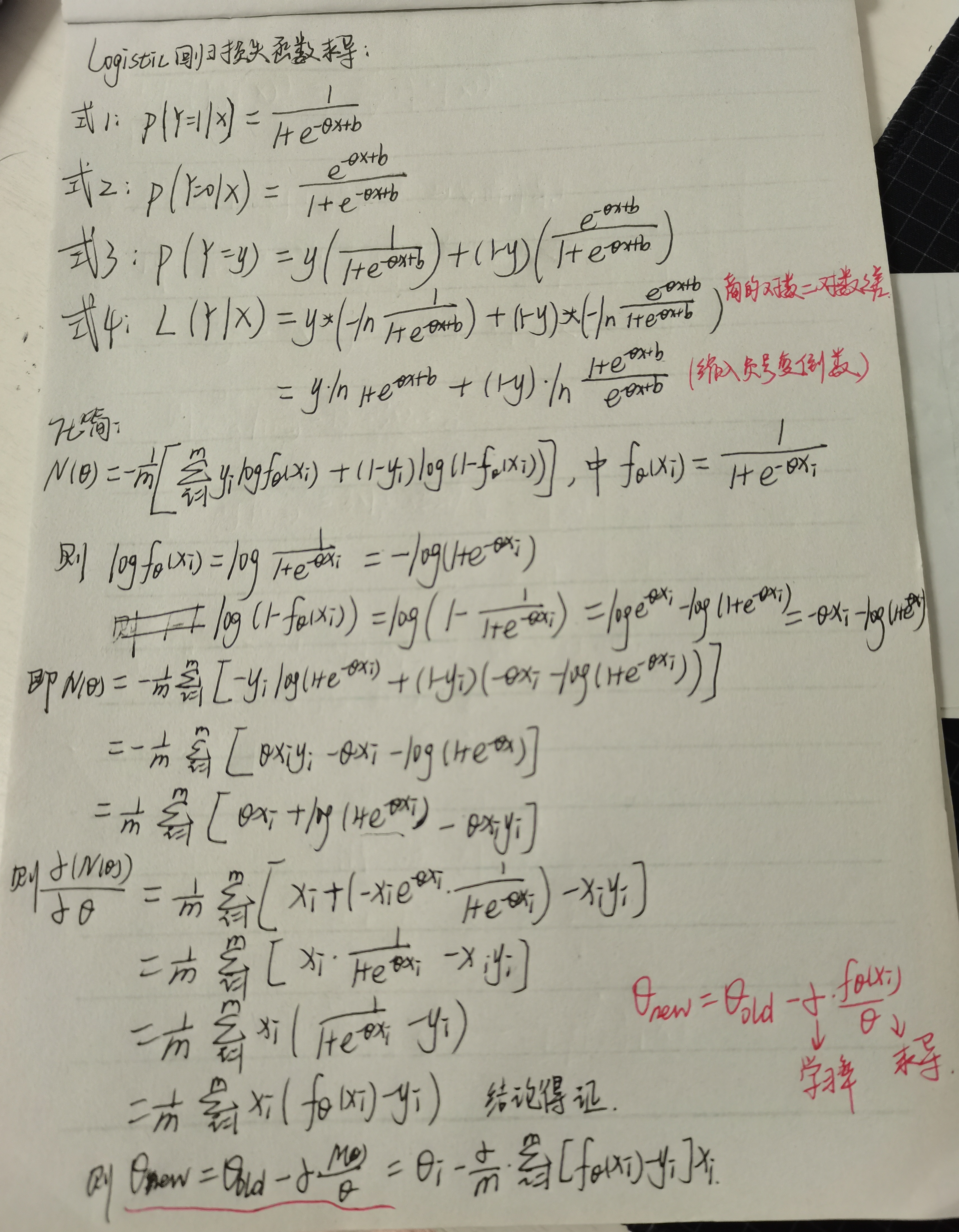
I Manual push to achieve logistic regression gradient descent

II Classification of iris data set by logistic regression

     1. Introduction to iris data set

     2. What is a linear classifier

     3. Main steps of designing linear classifier

     4. Rough definition of logistic regression

     5. In logistic regression model sklearn Use of

     6. Implementation of linear multi classification

     7. Related code

Zhengwen

I Manual push to achieve logistic regression gradient descent (picture below)

II Classification of iris data set by logistic regression

       1. Introduction to iris dataset

Iris data set is a classic data set for entry. Iris data set is a commonly used classification experimental data set, which was collected and sorted by Fisher,1936. Iris, also known as iris flower data set, is a kind of data set for multivariate analysis. Iris iris data set is} a classic data set. There are 150 records in 3 categories, 50 data in each category, and each record has four signs.            2. Introduction to linear classifier

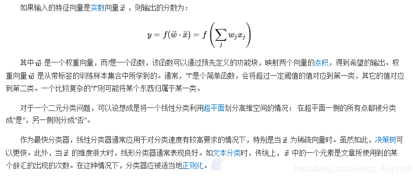
Linear classifier uses a "hyperplane" to separate positive and negative samples, such as:

(1) the positive and negative samples on the two-dimensional plane are classified by a straight line;
   (2) positive and negative samples in three-dimensional space are classified by a plane;
   (3) positive and negative samples in N-dimensional space are classified by a hyperplane;
   common linear classifiers include LR, Bayesian classification, single-layer perceptron, linear regression, SVM (linear kernel), etc

III Main steps of designing linear classifier

         ①. Collect a set of samples with category marks X={x1,x2,..., xN}
         ②. A criterion function J is determined as needed, its value reflects the performance of the classifier, and its extreme value solution corresponds to the "best" decision
         ③. The extremum solutions w * and w0 * of criterion function J are obtained by optimization technology, so as to determine the discriminant function and complete the classifier design
         ④. Obtain the linear discriminant function g(x)=wT+w0 or g(x)=a*Ty. For the unknown sample x, calculate g(x) and judge its category

IV Rough definition of logistic regression
Logistic Regression is used to deal with the regression problem in which the dependent variable is classified variable. The common problems are dichotomous and binomial distribution problems. It can also deal with multi classification problems (actually a probability model)

V Use of Sklearn in logistic regression model

        1). Import model

from sklearn.linear_model import LogisticRegression  #Import logistic regression model 

       2). fit() training} note: call the method of fit(x,y) to train the model, where x is the attribute of the data and Y is the type

clf = LogisticRegression()
print(clf)
clf.fit(train_feature,label)

      3). Prediction (prediction with trained model)

predict['label'] = clf.predict(predict_feature)

Vi Implementation of linear multi classification

      1). Linear classification using Jupyter Notebook (Anaconda)

      2). Multi classification linear coding

① import the required function library

#Import the required function library
import numpy as np
from sklearn.linear_model import LogisticRegression
import matplotlib.pyplot as plt
import matplotlib as mpl
from sklearn import datasets
from sklearn import preprocessing
import pandas as pd
from sklearn.preprocessing import StandardScaler
from sklearn.pipeline import Pipeline

② obtain iris data set

# Get the required dataset
iris=datasets.load_iris()
#There are four columns of data in each row, and each column is mapped to a feature_ Corresponding value in names
X=iris.data
print(X)
#The classification result value corresponding to each row of data (that is, the label value of each row of data) is [0,1,2]
Y=iris.target
print(Y)

③ data processing

#Normalization processing
X = StandardScaler().fit_transform(X)
print(X)

④ training model (using fit() function for training)

lr = LogisticRegression()   # Logistic regression model
lr.fit(X, Y)        # Calculate the regression parameters according to the data [x,y]

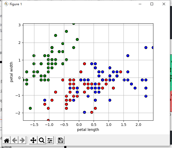
⑤ drawing graph (scatter diagram)

N, M = 500, 500     # How many values are sampled horizontally and vertically
x1_min, x1_max = X[:, 0].min(), X[:, 0].max()   # Range of column 0
x2_min, x2_max = X[:, 1].min(), X[:, 1].max()   # Range of column 1
t1 = np.linspace(x1_min, x1_max, N)
t2 = np.linspace(x2_min, x2_max, M)
x1, x2 = np.meshgrid(t1, t2)                    # Generate mesh sample points
x_test = np.stack((x1.flat, x2.flat), axis=1)   # Test point

cm_light = mpl.colors.ListedColormap(['#77E0A0', '#FF8080', '#A0A0FF'])
cm_dark = mpl.colors.ListedColormap(['g', 'r', 'b'])
y_hat = lr.predict(x_test)       # Estimate
y_hat = y_hat.reshape(x1.shape)                 # Make it the same as the entered shape
plt.pcolormesh(x1, x2, y_hat, cmap=cm_light)     # Display of predicted values
plt.scatter(X[:, 0], X[:, 1], c=Y.ravel(), edgecolors='k', s=50, cmap=cm_dark)    
plt.xlabel('petal length')
plt.ylabel('petal width')
plt.xlim(x1_min, x1_max)
plt.ylim(x2_min, x2_max)
plt.grid()
plt.show()

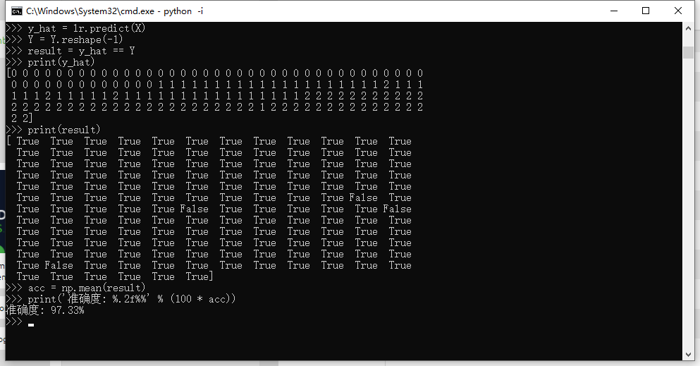
⑥ prediction model

y_hat = lr.predict(X)
Y = Y.reshape(-1)
result = y_hat == Y
print(y_hat)
print(result)
acc = np.mean(result)
print('Accuracy: %.2f%%' % (100 * acc))

⑦ complete code and result display

Code line

#Import related packages
import numpy as np
from sklearn.linear_model import LogisticRegression
import matplotlib.pyplot as plt
import matplotlib as mpl
from sklearn import datasets
from sklearn import preprocessing
import pandas as pd
from sklearn.preprocessing import StandardScaler
from sklearn.pipeline import Pipeline
# Get the required dataset
iris = datasets.load_iris()
#There are four columns of data in each row, and each column is mapped to a feature_ Corresponding value in names
X = iris.data
print(X)
#The classification result value corresponding to each row of data (that is, the label value of each row of data) is [0,1,2]
Y = iris.target
print(Y)
#Normalization processing
X = StandardScaler().fit_transform(X)
print(X)
lr = LogisticRegression()   # Logistic regression model
lr.fit(X, Y)        # Calculate the regression parameters according to the data [x,y]
N, M = 500, 500     # How many values are sampled horizontally and vertically
x1_min, x1_max = X[:, 0].min(), X[:, 0].max()   # Range of column 0
x2_min, x2_max = X[:, 1].min(), X[:, 1].max()   # Range of column 1
t1 = np.linspace(x1_min, x1_max, N)
t2 = np.linspace(x2_min, x2_max, M)
x1, x2 = np.meshgrid(t1, t2)                    # Generate mesh sample points
x_test = np.stack((x1.flat, x2.flat), axis=1)   # Test point
cm_light = mpl.colors.ListedColormap(['#77E0A0', '#FF8080', '#A0A0FF'])
cm_dark = mpl.colors.ListedColormap(['g', 'r', 'b'])
y_hat = lr.predict(x_test)       # Estimate
y_hat = y_hat.reshape(x1.shape)                 # Make it the same as the entered shape
plt.pcolormesh(x1, x2, y_hat, cmap=cm_light)     # Display of predicted values
plt.scatter(X[:, 0], X[:, 1], c=Y.ravel(), edgecolors='k', s=50, cmap=cm_dark)
plt.xlabel('petal length')
plt.ylabel('petal width')
plt.xlim(x1_min, x1_max)
plt.ylim(x2_min, x2_max)
plt.grid()
plt.show()
y_hat = lr.predict(X)
Y = Y.reshape(-1)
result = y_hat == Y
print(y_hat)
print(result)
acc = np.mean(result)
print('Accuracy: %.2f%%' % (100 * acc))

Result display

 

Machine learning -- linear multi classification of iris data set_ Harriet's blog - CSDN blog