This article mainly introduces the implementation of polynomial regression by artificial intelligence Python. Last time, we explained linear regression. This time, we focus on polynomial regression. You can refer to it
catalogue
1. Overview
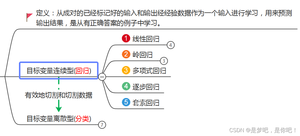
1.1 supervised learning
1.2 polynomial regression
2 Concept
3 case realization - Method 1
3.1 case analysis
3.2 code implementation
3.3 results
3.4 visualization
4 case realization - Method 2
4.1 code
4.2 results
4.3 visualization
1. Overview
1.1 supervised learning
1.2 polynomial regression
Last time we explained linear regression, this time we focus on polynomial regression.
Polynomial regression is a polynomial regression analysis method to study the relationship between a dependent variable and one or more independent variables. If there is only one independent variable, it is called univariate polynomial regression; If there are multiple independent variables, it is called multivariate polynomial regression.

(1) In univariate regression analysis, if the relationship between dependent variable y and independent variable x is nonlinear, but no appropriate function curve can be found to fit, univariate polynomial regression can be used.
(2) The greatest advantage of polynomial regression is that the measured points can be approximated by adding the higher-order term of x until satisfactory.
(3) In fact, polynomial regression can deal with quite a class of nonlinear problems. It plays an important role in regression analysis, because any function can be approximated by polynomials.
2 Concept
In the linear regression example mentioned earlier, a straight line is used to fit the linear relationship between data input and output. Unlike linear regression, polynomial regression uses a curve to fit the mapping relationship between the input and output of data.

3 case realization - Method 1
3.1 case analysis
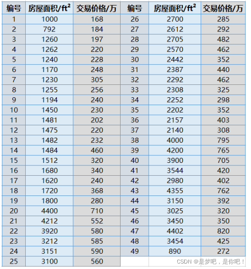
Application background: we have carried out linear regression according to the known house transaction price and house size, and then we can predict the transaction price of the example of known house size and unknown house transaction price. However, in practical application, such fitting is often not good enough, so we carry out polynomial regression on the data set.
Objective: to establish polynomial regression equation for house transaction information and predict house price according to the regression equation.
The transaction information includes the area of the house and the corresponding transaction price:
(1) The unit of house area is square feet (ft2)
(2) The unit of house transaction price is 10000
3.2 code implementation
import matplotlib.pyplot as plt
import numpy as np
from sklearn import linear_model
from sklearn.preprocessing import PolynomialFeatures
# Read dataset
datasets_X = []
datasets_Y = []
fr = open('Polynomial linear regression.csv','r')
lines = fr.readlines()
for line in lines:
items = line.strip().split(',')
datasets_X.append(int(items[0]))
datasets_Y.append(int(items[1]))
length = len(datasets_X)
datasets_X = np.array(datasets_X).reshape([length,1])
datasets_Y = np.array(datasets_Y)
minX = min(datasets_X)
maxX = max(datasets_X)
X = np.arange(minX,maxX).reshape([-1,1])
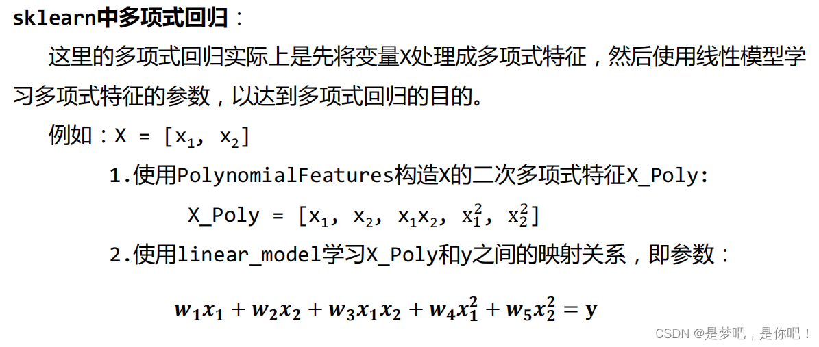
poly_reg = PolynomialFeatures(degree = 2) #degree=2 indicates the establishment of datasets_ Quadratic polynomial characteristic x of X_poly.
X_poly = poly_reg.fit_transform(datasets_X) #Construct the quadratic polynomial x of x using PolynomialFeatures_ poly
lin_reg_2 = linear_model.LinearRegression()
lin_reg_2.fit(X_poly, datasets_Y) #Then create a linear regression and use the linear_model to learn X_ Mapping relationship between poly and y
print(X_poly)
print(lin_reg_2.predict(poly_reg.fit_transform(X)))
print('Coefficients:', lin_reg_2.coef_) #View regression equation coefficients (k)
print('intercept:', lin_reg_2.intercept_) ##View intercept of regression equation (b)
print('the model is y={0}+({1}*x)+({2}*x^2)'.format(lin_reg_2.intercept_,lin_reg_2.coef_[0],lin_reg_2.coef_[1]))
# Display in image
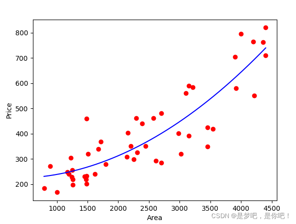
plt.scatter(datasets_X, datasets_Y, color = 'red') #scatter function is used to draw data points. Here, it means to draw data points in red;
#plot function is used to draw regression lines. Similarly, X needs to be processed into polynomial features first;
plt.plot(X, lin_reg_2.predict(poly_reg.fit_transform(X)), color = 'blue')
plt.xlabel('Area')
plt.ylabel('Price')
plt.show()
3.3 results
[[1.0000000e+00 1.0000000e+03 1.0000000e+06]
[1.0000000e+00 7.9200000e+02 6.2726400e+05]
[1.0000000e+00 1.2600000e+03 1.5876000e+06]
[1.0000000e+00 1.2620000e+03 1.5926440e+06]
[1.0000000e+00 1.2400000e+03 1.5376000e+06]
[1.0000000e+00 1.1700000e+03 1.3689000e+06]
[1.0000000e+00 1.2300000e+03 1.5129000e+06]
[1.0000000e+00 1.2550000e+03 1.5750250e+06]
[1.0000000e+00 1.1940000e+03 1.4256360e+06]
[1.0000000e+00 1.4500000e+03 2.1025000e+06]
[1.0000000e+00 1.4810000e+03 2.1933610e+06]
[1.0000000e+00 1.4750000e+03 2.1756250e+06]
[1.0000000e+00 1.4820000e+03 2.1963240e+06]
[1.0000000e+00 1.4840000e+03 2.2022560e+06]
[1.0000000e+00 1.5120000e+03 2.2861440e+06]
[1.0000000e+00 1.6800000e+03 2.8224000e+06]
[1.0000000e+00 1.6200000e+03 2.6244000e+06]
[1.0000000e+00 1.7200000e+03 2.9584000e+06]
[1.0000000e+00 1.8000000e+03 3.2400000e+06]
[1.0000000e+00 4.4000000e+03 1.9360000e+07]
[1.0000000e+00 4.2120000e+03 1.7740944e+07]
[1.0000000e+00 3.9200000e+03 1.5366400e+07]
[1.0000000e+00 3.2120000e+03 1.0316944e+07]
[1.0000000e+00 3.1510000e+03 9.9288010e+06]
[1.0000000e+00 3.1000000e+03 9.6100000e+06]
[1.0000000e+00 2.7000000e+03 7.2900000e+06]
[1.0000000e+00 2.6120000e+03 6.8225440e+06]
[1.0000000e+00 2.7050000e+03 7.3170250e+06]
[1.0000000e+00 2.5700000e+03 6.6049000e+06]
[1.0000000e+00 2.4420000e+03 5.9633640e+06]
[1.0000000e+00 2.3870000e+03 5.6977690e+06]
[1.0000000e+00 2.2920000e+03 5.2532640e+06]
[1.0000000e+00 2.3080000e+03 5.3268640e+06]
[1.0000000e+00 2.2520000e+03 5.0715040e+06]
[1.0000000e+00 2.2020000e+03 4.8488040e+06]
[1.0000000e+00 2.1570000e+03 4.6526490e+06]
[1.0000000e+00 2.1400000e+03 4.5796000e+06]
[1.0000000e+00 4.0000000e+03 1.6000000e+07]
[1.0000000e+00 4.2000000e+03 1.7640000e+07]
[1.0000000e+00 3.9000000e+03 1.5210000e+07]
[1.0000000e+00 3.5440000e+03 1.2559936e+07]
[1.0000000e+00 2.9800000e+03 8.8804000e+06]
[1.0000000e+00 4.3550000e+03 1.8966025e+07]
[1.0000000e+00 3.1500000e+03 9.9225000e+06]
[1.0000000e+00 3.0250000e+03 9.1506250e+06]
[1.0000000e+00 3.4500000e+03 1.1902500e+07]
[1.0000000e+00 4.4020000e+03 1.9377604e+07]
[1.0000000e+00 3.4540000e+03 1.1930116e+07]
[1.0000000e+00 8.9000000e+02 7.9210000e+05]]
[231.16788093 231.19868474 231.22954958 ... 739.2018995 739.45285011
739.70386176]
Coefficients: [ 0.00000000e+00 -1.75650177e-02 3.05166076e-05]
intercept: 225.93740561055927
the model is y=225.93740561055927+(0.0*x)+(-0.017565017675036532*x^2)
3.4 visualization
4 case realization - Method 2
4.1 code
import matplotlib.pyplot as plt
from sklearn.preprocessing import PolynomialFeatures
from sklearn.pipeline import Pipeline
from sklearn.linear_model import LinearRegression
from sklearn.metrics import mean_squared_error, r2_score
import numpy as np
import pandas as pd
import warnings

warnings.filterwarnings(action="ignore", module="sklearn")

dataset = pd.read_csv('Polynomial linear regression.csv')
X = np.asarray(dataset.get('x'))
y = np.asarray(dataset.get('y'))

# Divide training set and test set
X_train = X[:-2]
X_test = X[-2:]
y_train = y[:-2]
y_test = y[-2:]

# fit_intercept is True
model1 = Pipeline([('poly', PolynomialFeatures(degree=2)), ('linear', LinearRegression(fit_intercept=True))])
model1 = model1.fit(X_train[:, np.newaxis], y_train)
y_test_pred1 = model1.named_steps['linear'].intercept_ + model1.named_steps['linear'].coef_[1] * X_test
print('while fit_intercept is True:................')
print('Coefficients: ', model1.named_steps['linear'].coef_)
print('Intercept:', model1.named_steps['linear'].intercept_)
print('the model is: y = ', model1.named_steps['linear'].intercept_, ' + ', model1.named_steps['linear'].coef_[1],
      '* X')
# Mean square error
print("Mean squared error: %.2f" % mean_squared_error(y_test, y_test_pred1))
# r2 score, between 0 and 1, the closer it is to 1, the better the model, and the closer it is to 0, the worse the model
print('Variance score: %.2f' % r2_score(y_test, y_test_pred1), '\n')

# fit_intercept is False
model2 = Pipeline([('poly', PolynomialFeatures(degree=2)), ('linear', LinearRegression(fit_intercept=False))])
model2 = model2.fit(X_train[:, np.newaxis], y_train)
y_test_pred2 = model2.named_steps['linear'].coef_[0] + model2.named_steps['linear'].coef_[1] * X_test + \
               model2.named_steps['linear'].coef_[2] * X_test * X_test
print('while fit_intercept is False:..........................................')
print('Coefficients: ', model2.named_steps['linear'].coef_)
print('Intercept:', model2.named_steps['linear'].intercept_)
print('the model is: y = ', model2.named_steps['linear'].coef_[0], '+', model2.named_steps['linear'].coef_[1], '* X + ',
      model2.named_steps['linear'].coef_[2], '* X^2')
# Mean square error
print("Mean squared error: %.2f" % mean_squared_error(y_test, y_test_pred2))
# r2 score, between 0 and 1, the closer it is to 1, the better the model, and the closer it is to 0, the worse the model
print('Variance score: %.2f' % r2_score(y_test, y_test_pred2), '\n')

plt.xlabel('x')
plt.ylabel('y')
# Draw a scatter diagram of the training set
plt.scatter(X_train, y_train, alpha=0.8, color='black')
# Draw model
plt.plot(X_train, model2.named_steps['linear'].coef_[0] + model2.named_steps['linear'].coef_[1] * X_train +
         model2.named_steps['linear'].coef_[2] * X_train * X_train, color='red',
         linewidth=1)
plt.show()
4.2 results
If you do not use the framework, you need to manually add high-order items to the data. With the framework, it is much more convenient. sklearn uses the {Pipeline} function to simplify this part of the preprocessing process.
When degree=1 in , PolynomialFeatures , the effect is the same as using , LinearRegression , and a linear model is obtained. When degree=2, it is a quadratic equation. If it is a univariate, it is a parabola, and if it is a bivariate, it is a paraboloid. and so on.
Here's a} fit_ The intercept parameter. Let's take a look at its function through an example.
When {fit_ coef when intercept = True_ The first value in is 0, intercept_ The value in is the actual intercept.
When fit_ coef when intercept is False_ The first value in is intercept_ The value in is 0.
As shown in the figure, the first part is fit_ When intercept is True, the second part is "fit"_ The result when intercept is False.
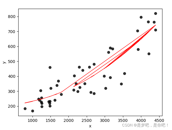
4.3 visualization
while fit_intercept is True:................
Coefficients:  [ 0.00000000e+00 -3.70858180e-04  2.78609637e-05]
Intercept: 204.25470490804574
the model is: y =  204.25470490804574  +  -0.00037085818009180454 * X
Mean squared error: 26964.95
Variance score: -3.61

while fit_intercept is False:..........................................
Coefficients:  [ 2.04254705e+02 -3.70858180e-04  2.78609637e-05]
Intercept: 0.0
the model is: y =  204.2547049080572 + -0.0003708581801012066 * X +  2.7860963722809286e-05 * X^2
Mean squared error: 7147.78
Variance score: -0.22
The above is the whole content of this article. I hope it can help you.