
Rimeng Society
AI AI:Keras PyTorch MXNet TensorFlow PaddlePaddle deep learning real combat (irregular update)
Encoder Decoder framework + Attention mechanism
Pytoch: building language models using Transformer
BahdanauAttention mechanism, LuongAttention mechanism
Attention mechanism, bmm operation
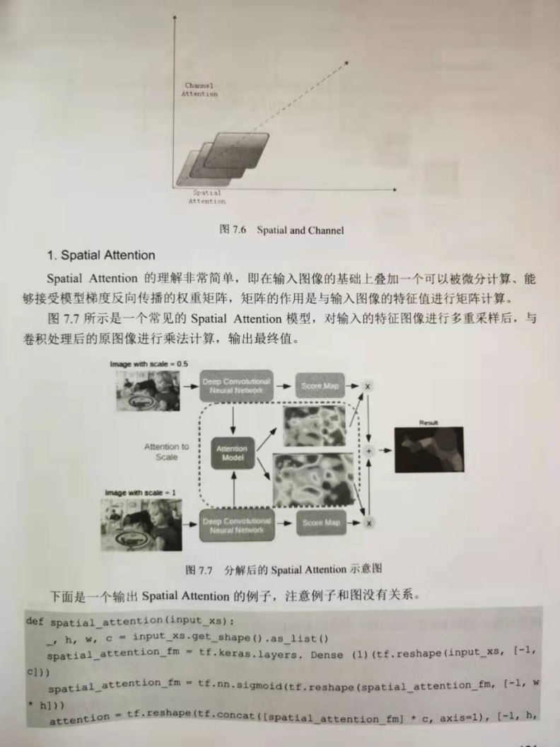
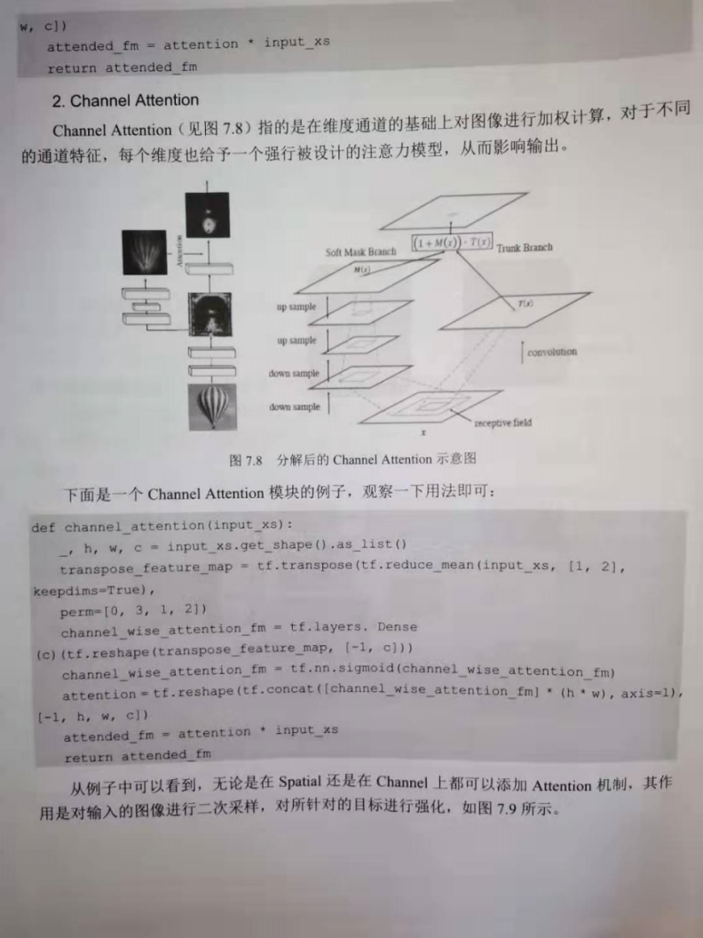
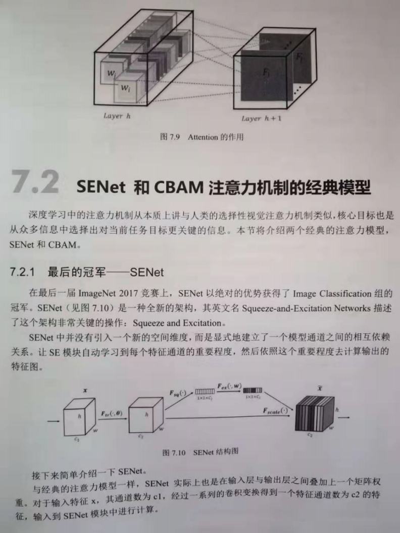
Attention mechanism SENet, CBAM
Note: This article is based on Transformer Programming practice of text emotion analysis based on( Encoder encoder-Decoder Decoder framework + Attention Attention mechanism + Positional Encoding Location code)
	The article implements Transformer of Model The type model is actually a modified special edition Transformer,because Transformer of Model Only implemented in the type model Encoder encoder,
	There is no corresponding implementation Decoder Decoder, and because of the current Transformer of Model The type model deals with classification tasks,
	So we only use Encoder Encoder to extract features, and finally fit the classification through the full connection layer network.
Back propagation, chain derivation
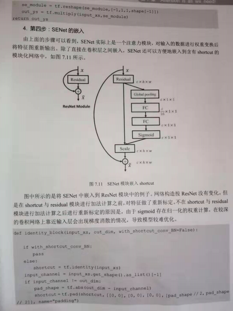
1.SENet modular
def SE_moudle(input_xs,reduction_ratio = 16.):
shape = input_xs.get_shape().as_list()
se_module = tf.reduce_mean(input_xs,[1,2])
#First density: shape[-1]/reduction_ratio: input_channel divided by reduction_ratio to lower the channel to the specified number of dimensions
se_module = tf.keras.layers.Dense(shape[-1]/reduction_ratio,activation=tf.nn.relu)(se_module)
#The second density: return to and input_ The same number of original dimensions as channel
se_module = tf.keras.layers.Dense(shape[-1], activation=tf.nn.relu)(se_module)
se_module = tf.nn.sigmoid(se_module)
se_module = tf.reshape(se_module,[-1,1,1,shape[-1]])
out_ys = tf.multiply(input_xs,se_module)
return out_ys
2.load SENet Modular Resnet
def identity_block(input_xs, out_dim, with_shortcut_conv_BN=False):
if with_shortcut_conv_BN:
pass
else:
#Returns the tensor with the same shape and content as input, that is, shortcut is equal to input_xs
shortcut = tf.identity(input_xs)
#Number of channel s input
input_channel = input_xs.get_shape().as_list()[-1]
#If the number of input channels is not equal to the number of output channels
if input_channel != out_dim:
#Calculate the absolute value of the number of output channels minus the number of input channels as the pad filling value
pad_shape = tf.abs(out_dim - input_channel)
#name="padding" means that the filling operation is given the name "padding". The default parameters mode='CONSTANT 'and constant are used_ Values = 0, indicating that the default value for filling is 0.
#The second parameter is the shape of padding filling: that is, the dimensions of batch, height and width are not filled, and pad is filled in the channel dimension_ Number of shapes / / 2.
shortcut = tf.pad(shortcut, [[0, 0], [0, 0], [0, 0], [pad_shape // 2, pad_shape // 2]], name="padding")
#The convolution kernels of the three Conv2D convolutions in the residual convolution block are 1x1, 3x3 and 1x1 respectively
conv = tf.keras.layers.Conv2D(filters=out_dim // 4, kernel_size=1, padding="SAME", activation=tf.nn.relu)(input_xs)
conv = tf.keras.layers.BatchNormalization()(conv)
conv = tf.keras.layers.Conv2D(filters=out_dim // 4, kernel_size=3, padding="SAME", activation=tf.nn.relu)(conv)
conv = tf.keras.layers.BatchNormalization()(conv)
conv = tf.keras.layers.Conv2D(filters=out_dim // 4, kernel_size=1, padding="SAME", activation=tf.nn.relu)(conv)
conv = tf.keras.layers.BatchNormalization()(conv)
#Now start loading the SENet module
#The returned dimension is [batch dimension, height, width, channel dimension]
shape = conv.get_shape().as_list()
#If the default parameter is keepdims=False, the dimension of the operation will not be retained. If keepdims=True, the dimension of the operation will be kept as 1.
#[batch dimension, height, width, channel dimension] after reduce_ Convert to [batch dimension, channel dimension] after mean
se_module = tf.reduce_mean(conv, [1, 2])
#First density: shape[-1]/reduction_ratio: input_channel divided by reduction_ratio to lower the channel to the specified number of dimensions
se_module = tf.keras.layers.Dense(shape[-1] / 16, activation=tf.nn.relu)(se_module)
#The second density: return to and input_ The same number of original dimensions as channel
se_module = tf.keras.layers.Dense(shape[-1], activation=tf.nn.relu)(se_module)
se_module = tf.nn.sigmoid(se_module)
#Re convert [batch dimension, channel dimension] to [batch dimension, height, width, channel dimension], i.e. [batch dimension, 1, 1, channel dimension]
se_module = tf.reshape(se_module, [-1, 1, 1, shape[-1]])
#multiply element multiplication: SENet module output value se_module and residual convolution output conv (i.e. SENet module input value conv)
se_module = tf.multiply(conv, se_module)
#Residual connection: the original input shortcut (i.e. input_xs) of the residual and the output value se of the SENet module_ Module
output_ys = tf.add(shortcut, se_module)
output_ys = tf.nn.relu(output_ys)
return output_ys
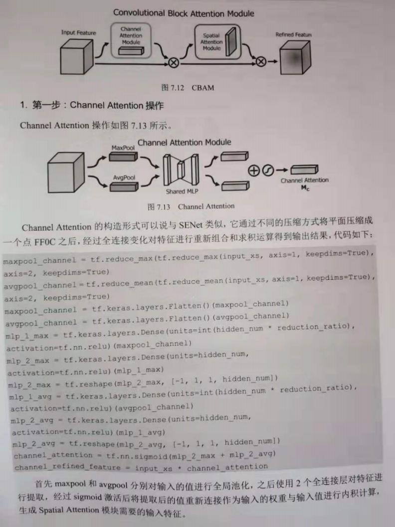
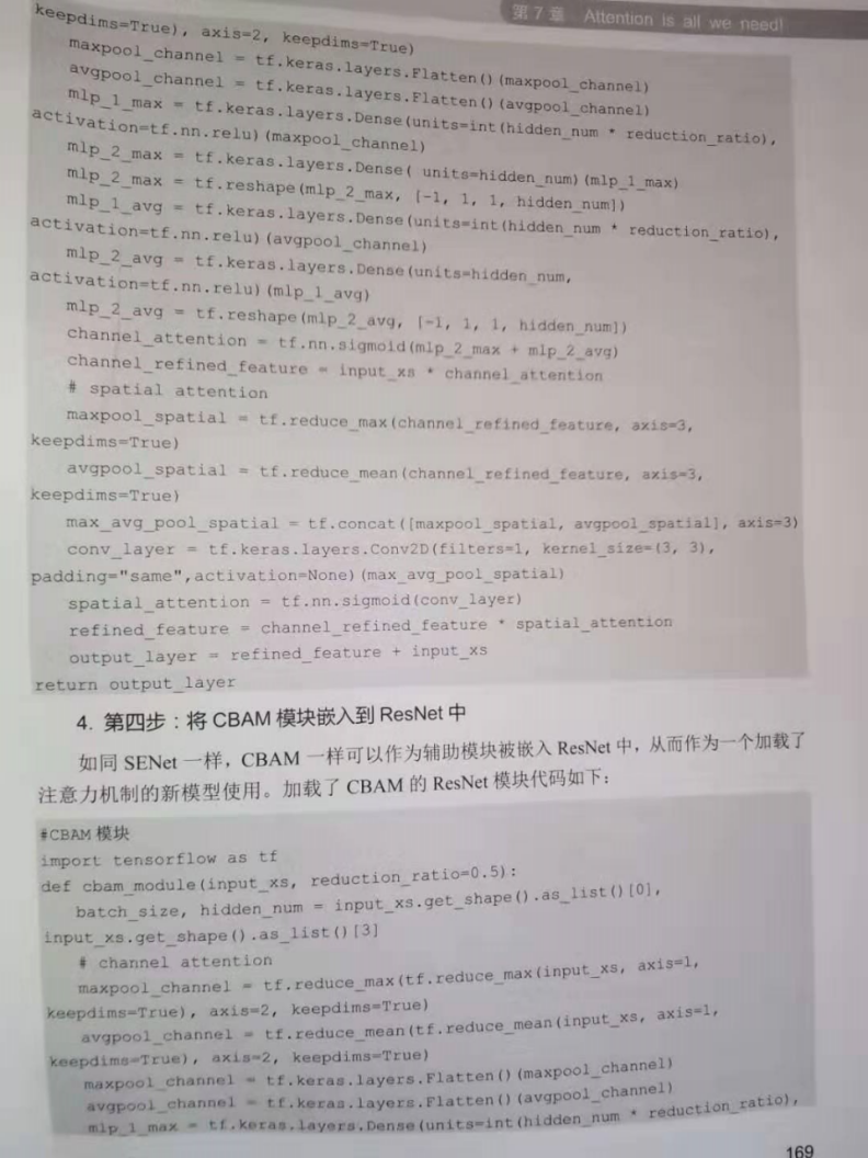
3.CBAM modular
def cbam_module(input_xs, reduction_ratio=0.5):
#The batch size and number of channels are obtained respectively, and the number of channels is used as the number of neurons in the hidden layer
batch_size, hidden_num = input_xs.get_shape().as_list()[0], input_xs.get_shape().as_list()[3]
### Step 1: Channel Attention modular ###
#1. If the default parameter is keepdims=False, the dimension of the operation will not be retained. If keepdims=True, the dimension of the operation will be kept as 1.
# Reduce twice in a row_ max/reduce_ Mean, in fact, first convert [batch dimension, height, width and channel dimension] to [batch dimension, 1, width and channel dimension],
# Then convert to [batch dimension, 1, 1, channel dimension].
#2. First, perform two operations: reduce_max and reduce_mean on the input data of the Channel Attention module.
maxpool_channel = tf.reduce_max(tf.reduce_max(input_xs, axis=1, keepdims=True), axis=2, keepdims=True)
avgpool_channel = tf.reduce_mean(tf.reduce_mean(input_xs, axis=1, keepdims=True), axis=2, keepdims=True)
maxpool_channel = tf.keras.layers.Flatten()(maxpool_channel)
avgpool_channel = tf.keras.layers.Flatten()(avgpool_channel)
#Two continuous full connection layers are used to extract the features after global pool (reduce_max).
#reduction_ The ratio is 0.5, that is, the number of neurons in the first full connection layer is half of the number of channels of input data, and then the number of neurons in the second full connection layer is restored to the number of channels of input data
mlp_1_max = tf.keras.layers.Dense(units=int(hidden_num * reduction_ratio), activation=tf.nn.relu)(maxpool_channel)
mlp_2_max = tf.keras.layers.Dense(units=hidden_num)(mlp_1_max)
#[batch dimension, 1, 1, channel dimension], the number of neurons in the hidden layer here is hidden_num is equal to the number of channels of input data
mlp_2_max = tf.reshape(mlp_2_max, [-1, 1, 1, hidden_num])
#Two continuous full connection layers are used to extract the features after reduce_mean.
#reduction_ The ratio is 0.5, that is, the number of neurons in the first full connection layer is half of the number of channels of input data, and then the number of neurons in the second full connection layer is restored to the number of channels of input data
mlp_1_avg = tf.keras.layers.Dense(units=int(hidden_num * reduction_ratio), activation=tf.nn.relu)(avgpool_channel)
mlp_2_avg = tf.keras.layers.Dense(units=hidden_num, activation=tf.nn.relu)(mlp_1_avg)
#[batch dimension, 1, 1, channel dimension], the number of neurons in the hidden layer here is hidden_num is equal to the number of channels of input data
mlp_2_avg = tf.reshape(mlp_2_avg, [-1, 1, 1, hidden_num])
#Sum the features of "reduce_max" and "reduce_mean", and then normalize them to 0-1 through sigmoid activation
channel_attention = tf.nn.sigmoid(mlp_2_max + mlp_2_avg)
#Calculate the inner product of the value "normalized by sigmoid activation" and the input data of the Channel Attention module, and the final calculated value is used as the input of the subsequent Spatial Attention module
channel_refined_feature = input_xs * channel_attention
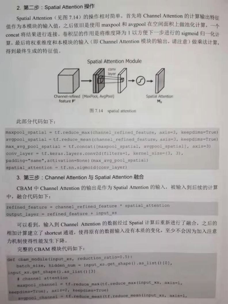
### Step 2: Spatial Attention modular ###
#1. First, take the output of the Channel Attention module as the input of the Spatial Attention module, and then perform two operations on the input data: reduce_max and reduce_mean.
#2. If the default parameter is keepdims=False, the dimension of the operation will not be retained. If keepdims=True, the dimension of the operation will be kept as 1.
#3. Reduce_max: convert [batch dimension, height, width, channel dimension] to [batch dimension, height, width, 1]
maxpool_spatial = tf.reduce_max(channel_refined_feature, axis=3, keepdims=True)
#Reduce_mean: convert [batch dimension, height, width, channel dimension] to [batch dimension, height, width, 1]
avgpool_spatial = tf.reduce_mean(channel_refined_feature, axis=3, keepdims=True)
#Merge the data after global pool (reduce_max) and average pool (reduce_mean) in the channel dimension, and finally convert it to [batch dimension, height, width, 2]
max_avg_pool_spatial = tf.concat([maxpool_spatial, avgpool_spatial], axis=3)
#The purpose is to reduce the dimension of the data to 1 so that the subsequent sigmoid can activate the normalization calculation
conv_layer = tf.keras.layers.Conv2D(filters=1, kernel_size=(3, 3), padding="same", activation=None)(max_avg_pool_spatial)
#Normalized to 0 to 1 by sigmoid activation
spatial_attention = tf.nn.sigmoid(conv_layer)
#The output channel of the Spatial Attention module_ refined_ Output of feature and Spatial Attention modules_ The inner product of attention is calculated,
#The final calculated value is used as the output value of CBAM attention mechanism module.
refined_feature = channel_refined_feature * spatial_attention
#Input the input value of CBAM attention mechanism module_ XS and output value refined_ Sum the features to get the final result
output_layer = refined_feature + input_xs
return output_layer
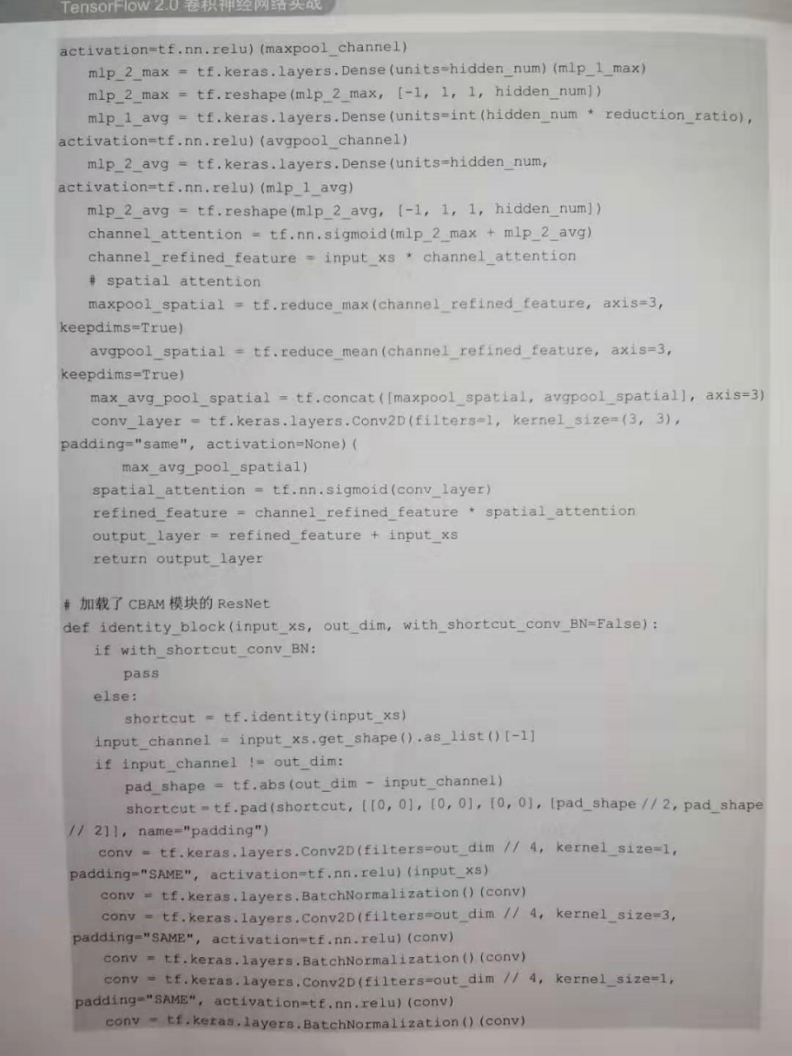
4.Loaded CBAM Modular Resnet
#CBAM module
import tensorflow as tf
def cbam_module(input_xs, reduction_ratio=0.5):
#The batch size and number of channels are obtained respectively, and the number of channels is used as the number of neurons in the hidden layer
batch_size, hidden_num = input_xs.get_shape().as_list()[0], input_xs.get_shape().as_list()[3]
### Step 1: Channel Attention modular ###
#1. If the default parameter is keepdims=False, the dimension of the operation will not be retained. If keepdims=True, the dimension of the operation will be kept as 1.
# Reduce twice in a row_ max/reduce_ Mean, in fact, first convert [batch dimension, height, width and channel dimension] to [batch dimension, 1, width and channel dimension],
# Then convert to [batch dimension, 1, 1, channel dimension].
#2. First, perform two operations: reduce_max and reduce_mean on the input data of the Channel Attention module.
maxpool_channel = tf.reduce_max(tf.reduce_max(input_xs, axis=1, keepdims=True), axis=2, keepdims=True)
avgpool_channel = tf.reduce_mean(tf.reduce_mean(input_xs, axis=1, keepdims=True), axis=2, keepdims=True)
maxpool_channel = tf.keras.layers.Flatten()(maxpool_channel)
avgpool_channel = tf.keras.layers.Flatten()(avgpool_channel)
#Two continuous full connection layers are used to extract the features after global pool (reduce_max).
#reduction_ The ratio is 0.5, that is, the number of neurons in the first full connection layer is half of the number of channels of input data, and then the number of neurons in the second full connection layer is restored to the number of channels of input data
mlp_1_max = tf.keras.layers.Dense(units=int(hidden_num * reduction_ratio), activation=tf.nn.relu)(maxpool_channel)
mlp_2_max = tf.keras.layers.Dense(units=hidden_num)(mlp_1_max)
#[batch dimension, 1, 1, channel dimension], the number of neurons in the hidden layer here is hidden_num is equal to the number of channels of input data
mlp_2_max = tf.reshape(mlp_2_max, [-1, 1, 1, hidden_num])
#Two continuous full connection layers are used to extract the features after reduce_mean.
#reduction_ The ratio is 0.5, that is, the number of neurons in the first full connection layer is half of the number of channels of input data, and then the number of neurons in the second full connection layer is restored to the number of channels of input data
mlp_1_avg = tf.keras.layers.Dense(units=int(hidden_num * reduction_ratio), activation=tf.nn.relu)(avgpool_channel)
mlp_2_avg = tf.keras.layers.Dense(units=hidden_num, activation=tf.nn.relu)(mlp_1_avg)
#[batch dimension, 1, 1, channel dimension], the number of neurons in the hidden layer here is hidden_num is equal to the number of channels of input data
mlp_2_avg = tf.reshape(mlp_2_avg, [-1, 1, 1, hidden_num])
#Sum the features of "reduce_max" and "reduce_mean", and then normalize them to 0-1 through sigmoid activation
channel_attention = tf.nn.sigmoid(mlp_2_max + mlp_2_avg)
#Calculate the inner product of the value "normalized by sigmoid activation" and the input data of the Channel Attention module, and the final calculated value is used as the input of the subsequent Spatial Attention module
channel_refined_feature = input_xs * channel_attention
### Step 2: Spatial Attention modular ###
#1. First, take the output of the Channel Attention module as the input of the Spatial Attention module, and then perform two operations on the input data: reduce_max and reduce_mean.
#2. If the default parameter is keepdims=False, the dimension of the operation will not be retained. If keepdims=True, the dimension of the operation will be kept as 1.
#3. Reduce_max: convert [batch dimension, height, width, channel dimension] to [batch dimension, height, width, 1]
maxpool_spatial = tf.reduce_max(channel_refined_feature, axis=3, keepdims=True)
#Reduce_mean: convert [batch dimension, height, width, channel dimension] to [batch dimension, height, width, 1]
avgpool_spatial = tf.reduce_mean(channel_refined_feature, axis=3, keepdims=True)
#Merge the data after global pool (reduce_max) and average pool (reduce_mean) in the channel dimension, and finally convert it to [batch dimension, height, width, 2]
max_avg_pool_spatial = tf.concat([maxpool_spatial, avgpool_spatial], axis=3)
#The purpose is to reduce the dimension of the data to 1 so that the subsequent sigmoid can activate the normalization calculation
conv_layer = tf.keras.layers.Conv2D(filters=1, kernel_size=(3, 3), padding="same", activation=None)(max_avg_pool_spatial)
#Normalized to 0 to 1 by sigmoid activation
spatial_attention = tf.nn.sigmoid(conv_layer)
#The output channel of the Spatial Attention module_ refined_ Output of feature and Spatial Attention modules_ The inner product of attention is calculated,
#The final calculated value is used as the output value of CBAM attention mechanism module.
refined_feature = channel_refined_feature * spatial_attention
#Input the input value of CBAM attention mechanism module_ XS and output value refined_ Sum the features to get the final result
output_layer = refined_feature + input_xs
return output_layer
# ResNet loaded with CBAM module
def identity_block(input_xs, out_dim, with_shortcut_conv_BN=False):
if with_shortcut_conv_BN:
pass
else:
#Returns the tensor with the same shape and content as input, that is, shortcut is equal to input_xs
shortcut = tf.identity(input_xs)
#Number of channel s input
input_channel = input_xs.get_shape().as_list()[-1]
#If the number of input channels is not equal to the number of output channels
if input_channel != out_dim:
#Calculate the absolute value of the number of output channels minus the number of input channels as the pad filling value
pad_shape = tf.abs(out_dim - input_channel)
#name="padding" means that the filling operation is given the name "padding". The default parameters mode='CONSTANT 'and constant are used_ Values = 0, indicating that the default value for filling is 0.
#The second parameter is the shape of padding filling: that is, the dimensions of batch, height and width are not filled, and pad is filled in the channel dimension_ Number of shapes / / 2.
shortcut = tf.pad(shortcut, [[0, 0], [0, 0], [0, 0], [pad_shape // 2, pad_shape // 2]], name="padding")
#The convolution kernels of the three Conv2D convolutions in the residual convolution block are 1x1, 3x3 and 1x1 respectively
conv = tf.keras.layers.Conv2D(filters=out_dim // 4, kernel_size=1, padding="SAME", activation=tf.nn.relu)(input_xs)
conv = tf.keras.layers.BatchNormalization()(conv)
conv = tf.keras.layers.Conv2D(filters=out_dim // 4, kernel_size=3, padding="SAME", activation=tf.nn.relu)(conv)
conv = tf.keras.layers.BatchNormalization()(conv)
conv = tf.keras.layers.Conv2D(filters=out_dim // 4, kernel_size=1, padding="SAME", activation=tf.nn.relu)(conv)
conv = tf.keras.layers.BatchNormalization()(conv)
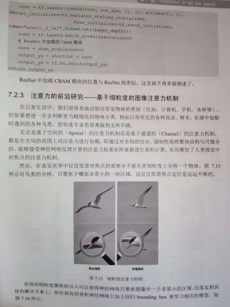
conv = tf.layers.conv2d(conv, out_dim, [1, 1], strides=[1, 1], kernel_initializer=tf.variance_scaling_initializer,
bias_initializer=tf.zeros_initializer, name="conv{}_2_1x1".format(str(layer_depth)))
conv = tf.layers.batch_normalization(conv)
# CBAM module loaded in ResNet
conv = cbam_module(conv)
#Residual connection: sum the original input shortcut (i.e. input_xs) of the residual with the output value conv of the CBAM module
output_ys = shortcut + conv
output_ys = tf.nn.relu(output_ys)
return output_ys
load SENet Modular ResNet-50
	def expand_dim_backend(self,x):
		x1 = K.reshape(x,(-1,1,256))
		print('x1:',x1)
		return x1

	def multiply(self,a):
		x = np.multiply(a[0], a[1])
		print('x:',x)
		return x

	def make_net_Res(self, encoding):
		# Input
		x = ZeroPadding1D(padding=3)(encoding)
		x = Conv1D(filters=64, kernel_size=7, strides=2, padding='valid', activation='relu')(x)
		x = BatchNormalization(axis=1, scale=True)(x)
		x_pool = MaxPooling1D(pool_size=3, strides=2, padding='same')(x)

	 	#RESNet_1
		x = Conv1D(filters=128, kernel_size=1, strides=1, padding='valid', activation='relu')(x_pool)
		x = BatchNormalization(axis=1, scale=True)(x)
		x = Conv1D(filters=128, kernel_size=3, strides=1, padding='valid', activation='relu')(x)
		x = BatchNormalization(axis=1, scale=True)(x)
		RES_1 = Conv1D(filters=256, kernel_size=1, strides=1, padding='valid', activation='relu')(x)
		x = BatchNormalization(axis=1, scale=True)(RES_1)

		# SENet
		squeeze = GlobalAveragePooling1D()(x)
		squeeze = Lambda(self.expand_dim_backend)(squeeze)
		excitation = Conv1D(filters=16, kernel_size=1, strides=1, padding='valid', activation='relu')(squeeze)
		excitation = Conv1D(filters=256, kernel_size=1, strides=1, padding='valid', activation='sigmoid')(excitation)
		x_pool_1 = Conv1D(filters=256, kernel_size=1, strides=1, padding='valid', activation='relu')(x_pool)
		x_pool_1 = BatchNormalization(axis=1, scale=True)(x_pool_1)

		#multiply element multiplication: SENet module output value excitation and residual convolution output res_ 1 (i.e. SENet module input value RES_1)
		scale = Lambda(self.multiply)([RES_1, excitation])
		res_1 = Concatenate(axis=1)([x_pool_1, scale])

		#RESNet_2
		x = Conv1D(filters=128, kernel_size=1, activation='relu')(res_1)
		x = BatchNormalization(axis=1, scale=True)(x)
		x = Conv1D(filters=128, kernel_size=3,  activation='relu')(x)
		x = BatchNormalization(axis=1, scale=True)(x)
		RES_2 = Conv1D(filters=256, kernel_size=1)(x)

		# SENet
		squeeze = GlobalAveragePooling1D()(RES_2)
		squeeze = Lambda(self.expand_dim_backend)(squeeze)
		excitation = Conv1D(filters=16, kernel_size=1, strides=1, padding='valid', activation='relu')(squeeze)
		excitation = Conv1D(filters=256, kernel_size=1, strides=1, padding='valid', activation='sigmoid')(excitation)

		#multiply element multiplication: SENet module output value excitation and residual convolution output res_ 2 (i.e. SENet module input value RES_2)
		scale = Lambda(self.multiply)([RES_2, excitation])
		x = Concatenate(axis=1)([res_1, scale])
		x = GlobalMaxPooling1D()(x)
		print('x:', x)
		output = Dense(1, activation='sigmoid')(x)
		return (output)