0 Introduction
multitasking learning: given m m m learning tasks, in which all or part of the tasks are related but not exactly the same. The goal of multi task learning is to use this method m m The knowledge contained in m tasks to help improve the performance of each task.
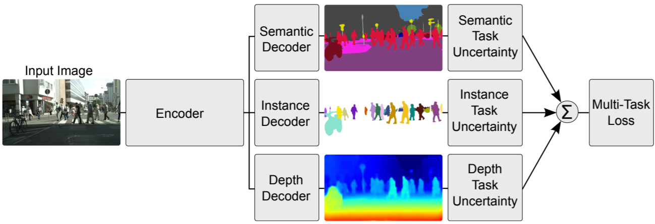
multitasking learning has many implementation paradigms, but we usually think that a model contains multiple objective functions to train and complete multiple tasks at the same time, which is multitasking learning in a broad sense. The following figure describes a typical multi task learning scenario. The model completes the tasks of semantic segmentation, instance segmentation and depth estimation at the same time.
L t o t a l = ∑ i w i L i L_{total} = \sum_{i}^{} w_iL_i Ltotal=i∑wiLi
in multi task learning, the training of the model is usually weighted by multiple loss functions to obtain the loss. Among them, the size of the loss function used by different tasks and the importance of the task need to be manually set, which makes us spend a lot of time adjusting the parameters or use the industry unified parameters (but whether it is optimal or not remains to be discussed). Therefore, it is considered whether the weight of each loss function can be automatically adjusted to liberate the training efficiency and even optimize the performance of the model.
this also leads to thinking: can this work be applied to single task multi output model (such as OCRNet, BiSeNetV2, U 2 ^2 2Net) or the weight adjustment parameter of single task mixed loss (for example, CELoss+LovaszSoftmaxLoss in semantic segmentation is usually 0.8 + 0.2).
the following is introduced by code.
1 data set definition
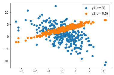
the following dataset defines two regression tasks, and we will use the same feature x x x completes two linear regressions y 1 y_1 y1 # and y 2 y_2 y2 task. The labels of these two tasks have different slopes, intercepts and variances (which can be modified by yourself).
import matplotlib.pyplot as plt
%matplotlib inline
import paddle
import numpy as np
class RegressionDataset(paddle.io.Dataset):
    def __init__(self, sample_nums):
        super(RegressionDataset, self).__init__()

        assert isinstance(sample_nums, int) and sample_nums > 0
        self.sample_nums = sample_nums
        self.x = np.random.randn(self.sample_nums, 1)
        self.y1 = self.generate_targets(w=-2, b=1, sigma=3.0)
        self.y2 = self.generate_targets(w=1.5, b=3, sigma=0.5)

    def __getitem__(self, idx):
        return (np.float32(self.x[idx]),
                np.float32(self.y1[idx]),
                np.float32(self.y2[idx]))

    def __len__(self):
        return self.sample_nums

    def generate_targets(self, w, b, sigma):
        return self.x * w + b + sigma * np.random.randn(self.sample_nums, 1)
np.random.seed(1024)
dataset = RegressionDataset(sample_nums=300)
plt.figure(figsize=(6, 4))
plt.scatter(dataset.x, dataset.y1)
plt.scatter(dataset.x, dataset.y2)
plt.legend([r'y1($\sigma=3$)', r'y2($\sigma=0.5$)'], loc=0)
plt.show()
2 model definition
a simple regression task model is defined here, but weight sharing is not adopted (it can be modified by yourself).
class MTLRegressionModel(paddle.nn.Layer):
    def __init__(self, in_nums, hidden_nums, out_nums):
        super(MTLRegressionModel, self).__init__()

        assert isinstance(in_nums, int) and in_nums > 0
        assert isinstance(hidden_nums, int) and hidden_nums > 0
        assert isinstance(out_nums, int) and out_nums > 0
        self.net1 = paddle.nn.Sequential(
            paddle.nn.Linear(in_features=in_nums, out_features=hidden_nums),
            paddle.nn.ReLU(),
            paddle.nn.Linear(in_features=hidden_nums, out_features=out_nums))
        self.net2 = paddle.nn.Sequential(
            paddle.nn.Linear(in_features=in_nums, out_features=hidden_nums),
            paddle.nn.ReLU(),
            paddle.nn.Linear(in_features=hidden_nums, out_features=out_nums))

    def forward(self, inputs):
        return [self.net1(inputs), self.net2(inputs)]
model = MTLRegressionModel(in_nums=1, hidden_nums=512, out_nums=1)
batch_size = 16
paddle.summary(model, input_size=(batch_size, 1))
for the above models, two mean square error functions mselos are usually selected, weighted as 1 : 1 1:1 1: 1, but is this weighting scheme optimal for model training?
3 same variance uncertainty
(Alex Kendall et al., 2018) It is proposed that using the same variance uncertainty to adjust the weight coefficient has achieved good results.
generally, there are two kinds of uncertainty in depth model modeling, namely cognitive uncertainty (under fitting, etc.) and accidental uncertainty (data information limitation, etc.), in which accidental uncertainty can be divided into homovariance uncertainty (data dependence) and heteroscedasticity uncertainty (task dependence). As shown in the introduction, multi task learning is usually different tasks of the same data set, so the uncertainty of the same variance is considered to measure the weight of the loss function.
the loss function based on the same variance uncertainty is derived from the perspective of regression and classification.
3.1 regression loss
output modeling (with observation noise):
p
(
y
∣
f
W
(
x
)
)
=
N
(
f
W
(
x
)
,
σ
2
)
p(y|f^W(x)) = \mathcal{N}(f^W(x),\sigma^2)
p(y∣fW(x))=N(fW(x),σ2)
log likelihood of maximized probability model:
log
p
(
y
∣
f
W
(
x
)
)
=
log
N
(
f
W
(
x
)
,
σ
2
)
=
log
(
1
2
π
σ
e
−
∣
∣
y
−
f
W
(
x
)
∣
∣
2
2
σ
2
)
∝
−
1
2
σ
2
∣
∣
y
−
f
W
(
x
)
∣
∣
2
−
log
σ
\log p(y|f^W(x)) = \log \mathcal{N}(f^W(x),\sigma^2) \\ = \log (\frac{1}{\sqrt{2\pi}\sigma} e^{-\frac{||y-f^W(x)||^2}{2\sigma^2}} ) \\ ∝ -\frac{1}{2\sigma^2}||y-f^W(x)||^2-\log \sigma
logp(y∣fW(x))=logN(fW(x),σ2)=log(2π
σ1e−2σ2∣∣y−fW(x)∣∣2)∝−2σ21∣∣y−fW(x)∣∣2−logσ
assuming that two regression tasks are carried out at the same time, there are the following output modeling:
p
(
y
1
,
y
2
∣
f
W
(
x
)
)
=
p
(
y
1
∣
f
W
(
x
)
)
⋅
p
(
y
2
∣
f
W
(
x
)
)
=
N
(
y
1
;
f
W
(
x
)
,
σ
1
2
)
⋅
N
(
y
2
;
f
W
(
x
)
,
σ
2
2
)
p(y_1,y_2|f^W(x)) = p(y_1|f^W(x))\cdot p(y_2|f^W(x)) \\ = \mathcal{N}(y_1;f^W(x),\sigma_1^2) \cdot \mathcal{N}(y_2;f^W(x),\sigma_2^2)
p(y1,y2∣fW(x))=p(y1∣fW(x))⋅p(y2∣fW(x))=N(y1;fW(x),σ12)⋅N(y2;fW(x),σ22)
maximizing the above log likelihood is equivalent to minimizing the following objective function:
L
(
W
,
σ
1
,
σ
2
)
=
−
log
(
p
(
y
1
,
y
2
∣
f
W
(
x
)
)
)
∝
1
2
σ
1
2
∣
∣
y
−
f
W
(
x
)
∣
∣
2
+
log
σ
1
+
1
2
σ
2
2
∣
∣
y
−
f
W
(
x
)
∣
∣
2
+
log
σ
2
=
1
2
σ
1
2
L
1
(
W
)
+
log
σ
1
+
1
2
σ
2
2
L
2
(
W
)
+
log
σ
2
\mathcal{L}(W,\sigma_1,\sigma_2) = -\log(p(y_1,y_2|f^W(x))) \\ ∝ \frac{1}{2\sigma_1^2}||y-f^W(x)||^2+\log \sigma_1+\frac{1}{2\sigma_2^2}||y-f^W(x)||^2+\log \sigma_2 \\= \frac{1}{2\sigma_1^2}\mathcal{L}_1(W) +\log \sigma_1+\frac{1}{2\sigma_2^2}\mathcal{L}_2(W) +\log \sigma_2
L(W,σ1,σ2)=−log(p(y1,y2∣fW(x)))∝2σ121∣∣y−fW(x)∣∣2+logσ1+2σ221∣∣y−fW(x)∣∣2+logσ2=2σ121L1(W)+logσ1+2σ221L2(W)+logσ2
noise σ \sigma σ Represents the uncertainty of the same variance, and the at the end l o g σ log \sigma log σ Equivalent to regular term.
3.2 classified losses
output modeling (introducing temperature coefficient)
σ
\sigma
σ, Gibbs distribution):
p
(
y
∣
f
W
(
x
)
)
=
softmax
(
1
σ
2
f
W
(
x
)
)
)
p(y|f^W(x)) = \text{softmax}(\frac{1}{\sigma^2}f^W(x)))
p(y∣fW(x))=softmax(σ21fW(x)))
log likelihood of classification model:
log
p
(
y
∣
f
W
(
x
)
)
=
log
softmax
(
1
σ
2
f
W
(
x
)
)
)
=
log
exp
(
1
σ
2
f
c
W
(
x
)
)
∑
c
exp
(
1
σ
2
f
c
W
(
x
)
)
=
1
σ
2
f
c
W
(
x
)
−
log
∑
c
exp
(
1
σ
2
f
c
W
(
x
)
)
=
1
σ
2
(
f
c
W
(
x
)
−
log
∑
c
exp
(
f
c
W
(
x
)
)
)
+
1
σ
2
log
∑
c
exp
(
f
c
W
(
x
)
)
−
log
∑
c
exp
(
1
σ
2
f
c
W
(
x
)
)
=
1
σ
2
(
log
exp
(
f
c
W
(
x
)
)
∑
c
exp
(
f
c
W
(
x
)
)
)
+
log
(
∑
c
exp
(
f
c
W
(
x
)
)
)
1
σ
2
−
log
∑
c
exp
(
1
σ
2
f
c
W
(
x
)
)
=
1
σ
2
(
log
exp
(
f
c
W
(
x
)
)
∑
c
exp
(
f
c
W
(
x
)
)
)
+
log
(
∑
c
exp
(
f
c
W
(
x
)
)
)
1
σ
2
−
log
∑
c
exp
(
1
σ
2
f
c
W
(
x
)
)
=
1
σ
2
(
log
softmax
(
f
W
(
x
)
)
)
+
log
(
∑
c
exp
(
f
c
W
(
x
)
)
)
1
σ
2
∑
c
exp
(
1
σ
2
f
c
W
(
x
)
)
\log p(y|f^W(x)) = \log \text{softmax}(\frac{1}{\sigma^2}f^W(x))) \\ = \log \frac{\exp(\frac{1}{\sigma^2}f_c^W(x))}{\sum_{c}^{}\exp(\frac{1}{\sigma^2}f_c^W(x))} \\ = \frac{1}{\sigma^2}f_c^W(x)-\log \sum_{c}^{}\exp(\frac{1}{\sigma^2}f_c^W(x)) \\ = \frac{1}{\sigma^2}(f_c^W(x)-\log \sum_{c}^{}\exp(f_c^W(x))) + \frac{1}{\sigma^2}\log \sum_{c}^{}\exp(f_c^W(x))-\log \sum_{c}^{}\exp(\frac{1}{\sigma^2}f_c^W(x)) \\ = \frac{1}{\sigma^2}(\log \frac{\exp(f_c^W(x))}{\sum_{c}^{}\exp(f_c^W(x))}) + \log (\sum_{c}^{}\exp(f_c^W(x)))^{\frac{1}{\sigma^2}}-\log \sum_{c}^{}\exp(\frac{1}{\sigma^2}f_c^W(x)) \\ = \frac{1}{\sigma^2}(\log \frac{\exp(f_c^W(x))}{\sum_{c}^{}\exp(f_c^W(x))}) + \log (\sum_{c}^{}\exp(f_c^W(x)))^{\frac{1}{\sigma^2}}-\log \sum_{c}^{}\exp(\frac{1}{\sigma^2}f_c^W(x)) \\ = \frac{1}{\sigma^2}(\log \text{softmax}(f^W(x))) + \log \frac{(\sum_{c}^{}\exp(f_c^W(x)))^{\frac{1}{\sigma^2}}}{ \sum_{c}^{}\exp(\frac{1}{\sigma^2}f_c^W(x))}
logp(y∣fW(x))=logsoftmax(σ21fW(x)))=log∑cexp(σ21fcW(x))exp(σ21fcW(x))=σ21fcW(x)−logc∑exp(σ21fcW(x))=σ21(fcW(x)−logc∑exp(fcW(x)))+σ21logc∑exp(fcW(x))−logc∑exp(σ21fcW(x))=σ21(log∑cexp(fcW(x))exp(fcW(x)))+log(c∑exp(fcW(x)))σ21−logc∑exp(σ21fcW(x))=σ21(log∑cexp(fcW(x))exp(fcW(x)))+log(c∑exp(fcW(x)))σ21−logc∑exp(σ21fcW(x))=σ21(logsoftmax(fW(x)))+log∑cexp(σ21fcW(x))(∑cexp(fcW(x)))σ21
assuming that regression and classification tasks are carried out at the same time, there are the following objective functions:
L
(
W
,
σ
1
,
σ
2
)
=
−
log
(
p
(
y
1
,
y
2
=
c
∣
f
W
(
x
)
)
)
=
−
log
N
(
y
1
;
f
W
(
x
)
,
σ
1
2
)
⋅
softmax
(
y
2
=
c
;
f
W
(
x
)
,
σ
2
2
)
=
1
2
σ
1
2
∣
∣
y
−
f
W
(
x
)
∣
∣
2
+
log
σ
1
−
log
p
(
y
2
=
c
;
f
W
(
x
)
,
σ
2
2
)
=
1
2
σ
1
2
∣
∣
y
−
f
W
(
x
)
∣
∣
2
+
log
σ
1
−
1
σ
2
2
(
log
softmax
(
f
W
(
x
)
)
)
−
log
(
∑
c
exp
(
f
c
W
(
x
)
)
)
1
σ
2
2
∑
c
exp
(
1
σ
2
2
f
c
W
(
x
)
)
=
1
2
σ
1
2
∣
∣
y
−
f
W
(
x
)
∣
∣
2
+
log
σ
1
+
1
σ
2
2
(
−
log
softmax
(
f
W
(
x
)
)
)
+
log
∑
c
exp
(
1
σ
2
2
f
c
W
(
x
)
)
(
∑
c
exp
(
f
c
W
(
x
)
)
)
1
σ
2
2
\mathcal{L}(W,\sigma_1,\sigma_2) = -\log(p(y_1,y_2=c|f^W(x))) \\ = -\log \mathcal{N}(y_1;f^W(x),\sigma_1^2)\cdot \text{softmax}(y_2=c;f^W(x),\sigma_2^2) \\ = \frac{1}{2\sigma_1^2}||y-f^W(x)||^2+\log \sigma_1-\log p(y_2=c;f^W(x),\sigma_2^2) \\ = \frac{1}{2\sigma_1^2}||y-f^W(x)||^2+\log \sigma_1 - \frac{1}{\sigma_2^2}(\log \text{softmax}(f^W(x))) - \log \frac{(\sum_{c}^{}\exp(f_c^W(x)))^{\frac{1}{\sigma_2^2}}}{ \sum_{c}^{}\exp(\frac{1}{\sigma_2^2}f_c^W(x))} \\ = \frac{1}{2\sigma_1^2}||y-f^W(x)||^2+\log \sigma_1 + \frac{1}{\sigma_2^2}(-\log \text{softmax}(f^W(x))) + \log \frac{ \sum_{c}^{}\exp(\frac{1}{\sigma_2^2}f_c^W(x))}{(\sum_{c}^{}\exp(f_c^W(x)))^{\frac{1}{\sigma_2^2}}}
L(W,σ1,σ2)=−log(p(y1,y2=c∣fW(x)))=−logN(y1;fW(x),σ12)⋅softmax(y2=c;fW(x),σ22)=2σ121∣∣y−fW(x)∣∣2+logσ1−logp(y2=c;fW(x),σ22)=2σ121∣∣y−fW(x)∣∣2+logσ1−σ221(logsoftmax(fW(x)))−log∑cexp(σ221fcW(x))(∑cexp(fcW(x)))σ221=2σ121∣∣y−fW(x)∣∣2+logσ1+σ221(−logsoftmax(fW(x)))+log(∑cexp(fcW(x)))σ221∑cexp(σ221fcW(x))
simplification: define regression loss as
L
1
(
W
)
=
∥
y
−
f
W
(
x
)
∥
2
\mathcal{L}_1(W)=\|y-f^W(x)\|^2
L1 (W) = ‖ y − fW(x) ‖ 2, the classification loss is
L
2
(
W
)
=
−
log
softmax
(
f
W
(
x
)
)
\mathcal{L}_2(W)=-\log \text{softmax}(f^W(x))
L2 (W) = − logsoftmax(fW(x)), approximate
1
σ
2
∑
c
exp
(
1
σ
2
2
f
c
W
(
x
)
)
≈
(
∑
c
exp
(
f
c
W
(
x
)
)
)
1
σ
2
2
\frac{1}{\sigma_2}\sum_{c}^{}\exp(\frac{1}{\sigma_2^2}f_c^W(x))≈(\sum_{c}^{}\exp(f_c^W(x)))^{\frac{1}{\sigma_2^2}}
σ 21∑cexp( σ 221fcW(x))≈(∑cexp(fcW(x))) σ 22 ^ 1. The approximate result of the above objective function is:
L ( W , σ 1 , σ 2 ) = 1 2 σ 1 2 L 1 ( W ) + log σ 1 + 1 σ 2 2 L 2 ( W ) + log σ 2 \mathcal{L}(W,\sigma_1,\sigma_2) = \frac{1}{2\sigma_1^2}\mathcal{L}_1(W)+\log \sigma_1+\frac{1}{\sigma_2^2}\mathcal{L}_2(W)+\log \sigma_2 L(W,σ1,σ2)=2σ121L1(W)+logσ1+σ221L2(W)+logσ2
3.3 conclusion
introduction of observation noise σ k \sigma_k σ k, has the following loss function:
L ( W , σ 1 , . . . , σ K ) = ∑ k = 1 K 1 2 σ k 2 L k ( W ) + log σ k \mathcal{L}(W,\sigma_1,...,\sigma_K) = \sum_{k=1}^{K}\frac{1}{2\sigma_k^2}\mathcal{L}_k(W)+\log \sigma_k L(W,σ1,...,σK)=k=1∑K2σk21Lk(W)+logσk
definition during training log σ 2 \log \sigma^2 log σ 2 is a trainable variable, which can limit the variation range and avoid the exception with denominator 0.
class MTLLoss(paddle.nn.Layer):
    def __init__(self, task_nums):
        super(MTLLoss, self).__init__()
        x = paddle.zeros([task_nums], dtype='float32')
        self.log_var2s = paddle.create_parameter(
            shape=x.shape,
            dtype=str(x.numpy().dtype),
            default_initializer=paddle.nn.initializer.Assign(x))

    def forward(self, logit_list, label_list):
        loss = 0
        for i in range(len(self.log_var2s)):
            mse = (logit_list[i] - label_list[i]) ** 2
            pre = paddle.exp(-self.log_var2s[i])
            loss += paddle.sum(pre * mse + self.log_var2s[i], axis=-1)
        return paddle.mean(loss)
mtl_loss = MTLLoss(task_nums=2)
paddle.summary(mtl_loss, input_size=[(batch_size, 1), (batch_size, 1)])
4 training parameters and training
it should be noted here that the optimizer should also load the parameters of the loss function model.
dataloader = paddle.io.DataLoader(
    dataset,
    batch_size=batch_size,
    shuffle=True)

parameters = model.parameters()
parameters.append(*mtl_loss.parameters())
optimizer = paddle.optimizer.Adam(
    learning_rate=0.0003,
    parameters=parameters)
start training, try 1500 rounds, and save the loss of each round and two trainable parameters.
loss_list, param_list = [], []
for epoch in range(1, 1501):
    model.train()
    loss_per_epoch = 0
    for x, y1, y2 in dataloader:
        logit_list = model(x)
        loss = mtl_loss(logit_list, [y1, y2])

        loss.backward()
        optimizer.step()
        optimizer.clear_grad()

        loss_per_epoch += loss.numpy()[0]

    loss_list.append(loss_per_epoch / len(dataset))
    param_list.append(mtl_loss.log_var2s.numpy())
5 training results
draw < loss change curve > and < same variance parameter change curve > below.
plt.figure(figsize=(6, 8))
plt.subplot(211)
plt.title('train loss')
plt.plot(loss_list)

plt.subplot(212)
sigma_list = np.sqrt(np.exp(param_list))
plt.title(r'$\sigma_k$: ' + f'{sigma_list[-1]}')
plt.plot(sigma_list[:, 0])
plt.plot(sigma_list[:, 1])
plt.legend([r'$\sigma_1$', r'$\sigma_2$'])

plt.tight_layout()
plt.show()
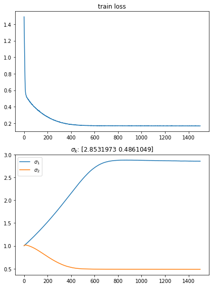
it can be observed that the training tends to converge in about 800 rounds.
re predict on the training set to obtain the fitted scatter points.
pred_list = []
for x, y1, y2 in dataset:
    x = paddle.to_tensor(x, dtype='float32')
    x = paddle.expand(x, shape=(1, 1))
    logit_list = model(x)
    logit_list = [paddle.squeeze(item).numpy() for item in logit_list]
    pred_list.append(logit_list)
pred_list = np.array(pred_list)
plt.figure(figsize=(6, 6))
plt.scatter(dataset.x, dataset.y1)
plt.scatter(dataset.x, dataset.y2)
plt.scatter(dataset.x, pred_list[:, 0])
plt.scatter(dataset.x, pred_list[:, 1])
plt.legend(
    [r'y1($\sigma=3$)',
     r'y2($\sigma=0.5$)',
     'pred_y1(σ=%0.4f)' % sigma_list[-1][0],
     'pred_y2(σ=%.4f)' % sigma_list[-1][1]],
    loc=0)
plt.show()
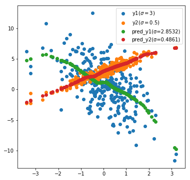
it is worth mentioning that: trainable parameters( p r e d _ y ∗ pred\_y* pred_y *) and the Gaussian distribution variance we set( y ∗ y* y *) is very close. If you add training samples, it may be closer. You might as well experiment by yourself.
6 PaddleSeg mixing loss
(Lukas Liebel et al., 2018) It is pointed out that the auxiliary task can optimize the training speed and network performance, and improve the above methods to prevent the training loss from becoming negative (in fact, this is different from our choice) l o g σ 2 log\ \sigma ^2 log σ 2 is similar to the training parameter. Here, 1 is added to the regularization term):
L c o m b ( x , y T , y T ′ ; ω T ) = ∑ τ ∈ T L τ ( x , y τ , y τ ′ ; ω τ ) ⋅ c τ \mathrm{L}_{\mathrm{comb}}\left(x, y_{\mathcal{T}}, y_{\mathcal{T}}^{\prime} ; \omega_{\mathcal{T}}\right)=\sum_{\tau \in \mathcal{T}} \mathrm{L}_{\tau}\left(x, y_{\tau}, y_{\tau}^{\prime} ; \omega_{\tau}\right) \cdot c_{\tau} Lcomb(x,yT,yT′;ωT)=τ∈T∑Lτ(x,yτ,yτ′;ωτ)⋅cτ
L T ( x , y T , y T ′ ; ω T ) = ∑ τ ∈ T 1 2 ⋅ c τ 2 ⋅ L τ ( x , y τ , y τ ′ ; ω τ ) + ln ( 1 + c τ 2 ) \begin{aligned} \mathrm{L}_{\mathcal{T}}\left(x, y_{\mathcal{T}}, y_{\mathcal{T}}^{\prime} ; \omega_{\mathcal{T}}\right)=& \sum_{\tau \in \mathcal{T}} \frac{1}{2 \cdot c_{\tau}^{2}} \cdot \mathrm{L}_{\tau}\left(x, y_{\tau}, y_{\tau}^{\prime} ; \omega_{\tau}\right) +\ln \left(1+c_{\tau}^{2}\right) \end{aligned} LT(x,yT,yT′;ωT)=τ∈T∑2⋅cτ21⋅Lτ(x,yτ,yτ′;ωτ)+ln(1+cτ2)
try to apply this method to the parameter adjustment of the weight of the mixed loss function. Take PaddleSeg as an example to write the loss function. Pay attention to loading the parameters of the loss function when initializing the optimizer. The following code groups have been run twice to get the comparison results, namely self weight loss and fixed weight. Pay attention to saving the path when running.
!pip install paddleseg==2.4.0
import numpy as np
import random
import paddle
import paddleseg
import paddleseg.transforms as T

from paddleseg.cvlibs import manager
from paddleseg.datasets import OpticDiscSeg
from paddleseg.models import MixedLoss, CrossEntropyLoss, DiceLoss
random.seed(1024)
paddle.seed(1024)
np.random.seed(1024)
transforms = [T.Resize(target_size=(512, 512)), T.Normalize()]

train_dataset = OpticDiscSeg(
    dataset_root='data/optic_disc_seg',
    transforms=transforms,
    mode='train')
val_dataset = OpticDiscSeg(
    dataset_root='data/optic_disc_seg',
    transforms=transforms,
    mode='val')
test_dataset = OpticDiscSeg(
    dataset_root='data/optic_disc_seg',
    transforms=transforms,
    mode='val')
model = paddleseg.models.HarDNet(num_classes=2)
note: the above only deduces the cross entropy and mean square error. If it is applied, it can be deduced in the same way as other losses, but we still try this method for Dice Loss first.
@manager.LOSSES.add_component
class AutoWeightedLoss(paddle.nn.Layer):
    def __init__(self, losses):
        super(AutoWeightedLoss, self).__init__()

        self.losses = losses
        x = paddle.ones(shape=[len(losses)], dtype='float32')
        self.coefs = paddle.create_parameter(
            shape=x.shape,
            dtype=str(x.numpy().dtype),
            attr=paddle.ParamAttr(
                initializer=paddle.nn.initializer.Assign(x),
                regularizer=None
            ))

    def forward(self, logits, labels):
        loss_sum = 0
        for i, loss in enumerate(self.losses):
            square = self.coefs[i] ** 2
            loss_sum += loss(logits, labels) / (2 * square) + paddle.log(1 + square)
        return loss_sum
use_auto_weighted_loss = True
parameters = model.parameters()

if use_auto_weighted_loss:
    losses = {
        'types': [AutoWeightedLoss([CrossEntropyLoss(), DiceLoss()])],
        'coef': [1]
    }
    parameters.append(*losses['types'][0].parameters())
else:
    losses = {
        'types': [MixedLoss([CrossEntropyLoss(), DiceLoss()], [0.8, 0.2])],
        'coef': [1]
    }
iters = 10000
train_batch_size = 4
learning_rate = 0.001

decayed_lr = paddle.optimizer.lr.PolynomialDecay(
    learning_rate=learning_rate,
    decay_steps=iters,
    end_lr=0.0)

optimizer = paddle.optimizer.AdamW(
    learning_rate=decayed_lr,
    parameters=parameters)
from paddleseg.core import train

train(
    train_dataset=train_dataset,
    val_dataset=val_dataset,

    model=model,
    optimizer=optimizer,
    losses=losses,

    iters=iters,
    batch_size=train_batch_size,

    save_interval=500,
    log_iters=100,
    num_workers=2,
    save_dir='output/hardnet_b4_10k_auto',
    use_vdl=False)
from paddleseg.core import evaluate

model = paddleseg.models.HarDNet(num_classes=2)
params_path = 'output/hardnet_b4_10k_auto/best_model/model.pdparams'
model_state_dict = paddle.load(params_path)
model.set_dict(model_state_dict)

evaluate(
    model,
    test_dataset,
    aug_eval=True,
    flip_horizontal=True,

model_state_dict = paddle.load(params_path)
model.set_dict(model_state_dict)

evaluate(
    model,
    test_dataset,
    aug_eval=True,
    flip_horizontal=True,
    flip_vertical=True)
print trainable parameters of automatic loss.
losses['types'][0].parameters()[0].numpy()
array([0.25268388, 0.45781416], dtype=float32)
< test set evaluation resu lt s >: the same learning rate strategy may be unfair to one party, and the effect of mixed use of Dice Loss without derivation needs to be verified.
| iter 20k | CE Loss+Dice Loss (auto) | CE Loss+Dice Loss (0.8:0.2) |
|---|---|---|
| mIoU | 0.8883 | 0.8752 |
| Dice | 0.9374 | 0.9291 |
| kappa | 0.8749 | 0.8581 |
7 Summary
this project introduces the difficulty of weight setting between different loss functions in multi task learning. Referring to the above two citations, it deduces the automatic weight setting method when cross entropy loss and mean square error loss are mixed from the perspective of CO variance uncertainty - taking it as a trainable parameter.
if you are interested, you can extend it to other losses.
as the author of the citation said, it doesn't always work, but I hope this article can help you~~