introduce
Generative model is an important model in unsupervised learning, which has attracted extensive attention in recent years. They can be defined as a kind of model, whose goal is to learn how to generate new samples from the same data set as the training data. In the training phase, the generation model attempts to solve the core task of density estimation. In density estimation, our model learns to construct an estimation - pmodel(x) - as similar as unobservable probability density function - pdata(x). It should be noted that the generation model should be able to generate new samples from the distribution, not just copy and paste existing samples. Once we have successfully trained our model, it can be used in a variety of applications, from various forms of reconstruction, such as image filling, coloring and super-resolution to art generation.
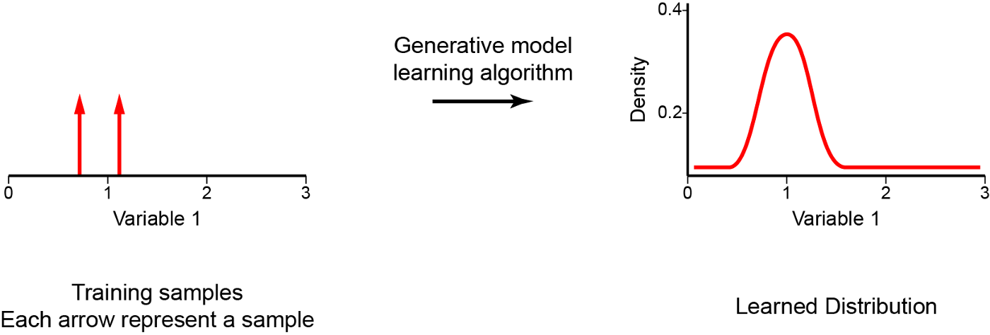
We can use several different methods to perform this probability density estimation, such as:
- The generation countermeasure network (GAN) uses the model to perform implicit density estimation. In this case, we train a model that can create samples from pmodel(x) without explicitly defining pmodel(x); The model learns a random process and uses the process to generate data, but does not provide the knowledge of observation probability or specify a conditional log likelihood function;
- Variational self encoder (VAE) uses explicit density estimation, but defines a difficult density function with potential variables. Therefore, in order to train the model, we derive and optimize the lower bound of likelihood (approximate density); We optimize the log likelihood of the data by maximizing the lower bound of evidence (ELBO);
- The autoregressive (AR) model creates an explicit density model that is easy to process to maximize the possibility of training data (processable density). For this reason, using these methods, it is easy to calculate the possibility of data observation and obtain the evaluation indicators of the generated model.
As mentioned above, autoregression is a practical method, which provides explicit modeling of likelihood function. However, to model data with multiple dimensions / characteristics, autoregressive model needs some additional conditions. First, the input space X needs to determine and sort its characteristics. This is why autoregressive models are usually used for time series with internal time steps. They can be used for images by defining, for example, the left pixel before the right pixel and the top pixel before the bottom pixel. Secondly, in order to easily model the joint distribution of features in data observation (p(x)), autoregressive method regards p(x) as the product of conditional distribution. Given the values of previous features, the autoregressive model uses the conditions of each feature to define the joint distribution. For example, the probability that a pixel in an image has a specific intensity value depends on the values of all previous pixels; The probability of an image (the joint distribution of all pixels) is the combination of the probabilities of all pixels. Therefore, the autoregressive model uses the chain rule to decompose the likelihood of data sample x into the product of one-dimensional distribution (the following equation). Decomposition transforms the joint modeling problem into a sequence problem, and learns to predict the next pixel given all the previously generated pixels.
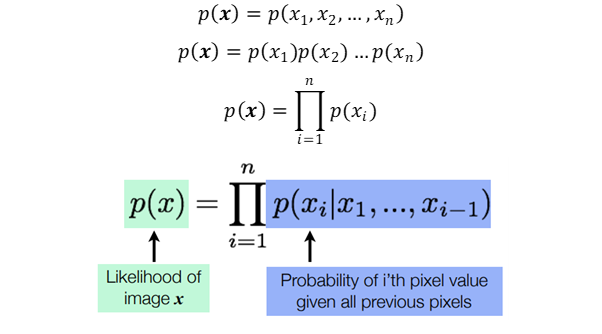
These conditions (i.e. determining the order and product of conditional distribution) are the main conditions for defining autoregressive models.
Now, the biggest challenge is to calculate these conditional likelihood p(x ᵢ x ₁,, X ᵢ x ₋). How do we define these complex distributions in an easy to handle and extensible expression model? One solution is to use general approximators, such as deep neural networks.
PixelCNN
DeepMind introduced PixelCNN (Oord et al., 2016) in 2016, which opened the most promising family of autoregressive generation models. Since then, it has been used to generate voice, video and high-resolution pictures.
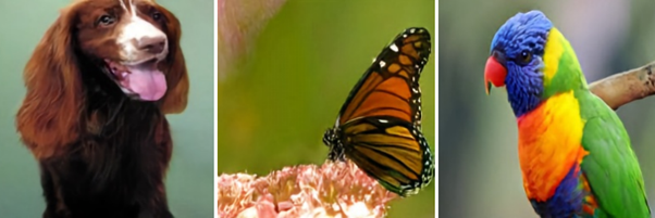
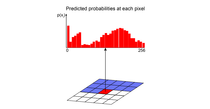
Pixel CNN is a deep neural network, which captures the dependency distribution between pixels in its parameters. It generates one pixel at a time in the image along two spatial dimensions.
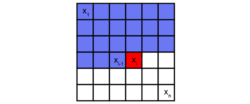
Pixel i (red) is defined by all previous pixels (blue). Pixel CNN can use the convolution layer along the depth neural network to model their correlation.
Using convolution operation, PixelCNN can learn the distribution of all pixels in the image in parallel. However, when determining the probability of a specific pixel, the receptive field of the standard convolution layer violates the sequential prediction of the autoregressive model. When processing the information of a central pixel, the convolution filter will consider all the pixels around it to calculate the output characteristic image, not just the front pixels. Therefore, a mask is needed to block the flow of information from pixels that have not been predicted.
Masked convolution layer
Masking can be done by zeroing all pixels that should not be considered. In our implementation, a mask with the same size as the convolution filter and values of 1 and 0 is created. Before convolution, this mask is multiplied by the weight tensor. In PixelCNN, there are two types of masks:
Mask type A: this mask applies only to the first volume layer. It restricts access to pixels by zeroing the center pixel in the mask. In this way, we guarantee that the model will not access the pixels it is about to predict (the red part in the figure below).
Mask type B: this mask is applied to all subsequent convolution layers, and the limitation of mask A is relaxed by allowing the connection from the pixel to itself. This is important for explaining the pixel prediction of the first layer.
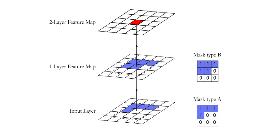
Mask A is only used for the first volume layer. Mask B is used for all other layers to allow information of pixel centered convolution operations to propagate along the network.
Here, we show a fragment that implements the mask using the Tensorflow 2.0 framework.
class MaskedConv2D(keras.layers.Layer):
    """Convolutional layers with masks.

    Convolutional layers with simple implementation of masks type A and B for
    autoregressive models.

    Arguments:
    mask_type: one of `"A"` or `"B".`
    filters: Integer, the dimensionality of the output space
        (i.e. the number of output filters in the convolution).
    kernel_size: An integer or tuple/list of 2 integers, specifying the
        height and width of the 2D convolution window.
        Can be a single integer to specify the same value for
        all spatial dimensions.
    strides: An integer or tuple/list of 2 integers,
        specifying the strides of the convolution along the height and width.
        Can be a single integer to specify the same value for
        all spatial dimensions.
        Specifying any stride value != 1 is incompatible with specifying
        any `dilation_rate` value != 1.
    padding: one of `"valid"` or `"same"` (case-insensitive).
    kernel_initializer: Initializer for the `kernel` weights matrix.
    bias_initializer: Initializer for the bias vector.
    """

    def __init__(self,
                 mask_type,
                 filters,
                 kernel_size,
                 strides=1,
                 padding='same',
                 kernel_initializer='glorot_uniform',
                 bias_initializer='zeros'):
        super(MaskedConv2D, self).__init__()

        assert mask_type in {'A', 'B'}
        self.mask_type = mask_type

        self.filters = filters
        self.kernel_size = kernel_size
        self.strides = strides
        self.padding = padding.upper()
        self.kernel_initializer = initializers.get(kernel_initializer)
        self.bias_initializer = initializers.get(bias_initializer)

    def build(self, input_shape):
        self.kernel = self.add_weight('kernel',
                                      shape=(self.kernel_size,
                                             self.kernel_size,
                                             int(input_shape[-1]),
                                             self.filters),
                                      initializer=self.kernel_initializer,
                                      trainable=True)

        self.bias = self.add_weight('bias',
                                    shape=(self.filters,),
                                    initializer=self.bias_initializer,
                                    trainable=True)

        center = self.kernel_size // 2

        mask = np.ones(self.kernel.shape, dtype=np.float32)
        mask[center, center + (self.mask_type == 'B'):, :, :] = 0.
        mask[center + 1:, :, :, :] = 0.

        self.mask = tf.constant(mask, dtype=tf.float32, name='mask')

    def call(self, input):
        masked_kernel = tf.math.multiply(self.mask, self.kernel)
        x = nn.conv2d(input,
                      masked_kernel,
                      strides=[1, self.strides, self.strides, 1],
                      padding=self.padding)
        x = nn.bias_add(x, self.bias)
        return x
Model architecture
Pixel CNN uses the following architecture: the first layer is mask convolution (type A) with 7x7 filters. Then, 15 residual blocks are used. Each block processes data using a combination of 3x3 convolution layers of mask type B and standard 1x1 convolution layers. Between each convolution layer, there is a nonlinear ReLU.
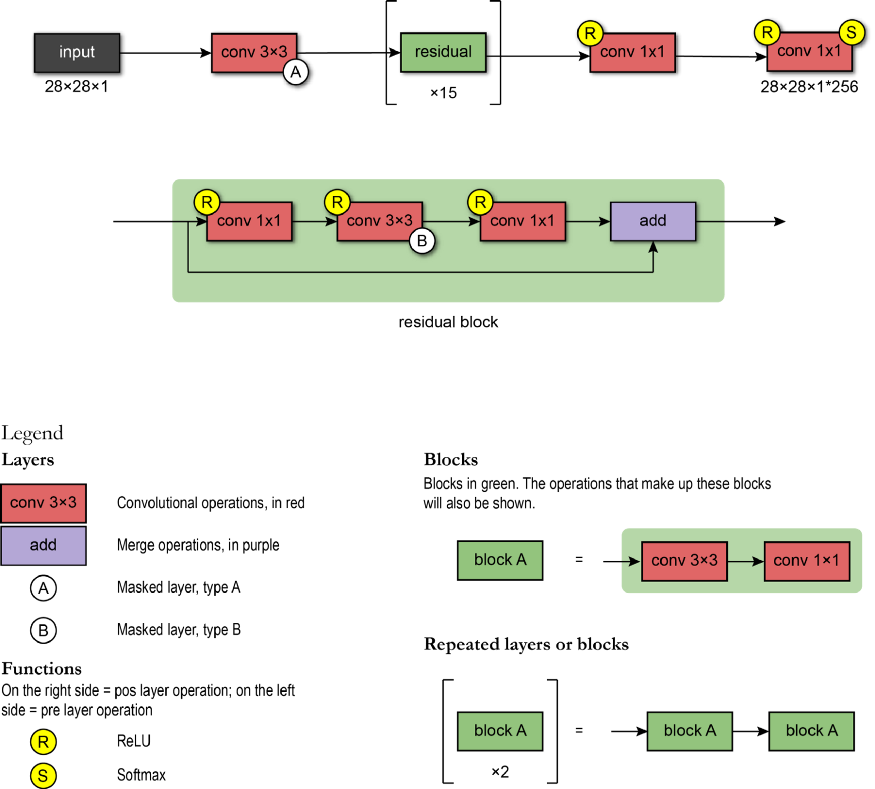
After the sequence block is the RELU-CONV-RELU-CONV layer, where CONV is a standard convolution with 1x1 filter. Then, the output layer is a softmax layer that predicts all possible values of pixels. The output of the model has the same format as the input image size (because we want the output value of each pixel) multiplied by the number of possible values (classified according to intensity levels, such as 256 intensity levels).
class ResidualBlock(keras.Model):
    """Residual blocks that compose pixelCNN

    Blocks of layers with 3 convolutional layers and one residual connection.
    Based on Figure 5 from [1] where h indicates number of filters.

    Refs:
    [1] - Oord, A. V. D., Kalchbrenner, N., & Kavukcuoglu, K. (2016). Pixel
     recurrent neural networks. arXiv preprint arXiv:1601.06759.
    """

    def __init__(self, h):
        super(ResidualBlock, self).__init__(name='')

        self.conv2a = keras.layers.Conv2D(filters=h, kernel_size=1, strides=1)
        self.conv2b = MaskedConv2D(mask_type='B', filters=h, kernel_size=3, strides=1)
        self.conv2c = keras.layers.Conv2D(filters=2 * h, kernel_size=1, strides=1)

    def call(self, input_tensor):
        x = nn.relu(input_tensor)
        x = self.conv2a(x)

        x = nn.relu(x)
        x = self.conv2b(x)

        x = nn.relu(x)
        x = self.conv2c(x)

        x += input_tensor
        return x

# Create PixelCNN model
inputs = keras.layers.Input(shape=(height, width, n_channel))
x = MaskedConv2D(mask_type='A', filters=128, kernel_size=7, strides=1)(inputs)

for i in range(15):
    x = ResidualBlock(h=64)(x)

x = keras.layers.Activation(activation='relu')(x)
x = keras.layers.Conv2D(filters=128, kernel_size=1, strides=1)(x)
x = keras.layers.Activation(activation='relu')(x)
x = keras.layers.Conv2D(filters=128, kernel_size=1, strides=1)(x)
x = keras.layers.Conv2D(filters=q_levels, kernel_size=1, strides=1)(x)

pixelcnn = keras.Model(inputs=inputs, outputs=x)
Pretreatment
The input value of PixelCNN is scaled to the range of [0, 1]. By quantifying the input value, the purpose of rapid convergence can be achieved.
The output target corresponds to a classification (integer) value indicating pixel intensity.
Model evaluation index
Pixel CNN is also a classification problem, so the model trains its parameters by maximizing the possibility of the target.

Most optimization problems can be defined as minimization problems, so the common technique is to convert the training target to the minimization of negative log likelihood (NLL).

Because p(x ᵢ| θ) Corresponding to the probability of softmax layer output, NLL is equivalent to the cross entropy loss function, a loss function commonly used in supervised learning. In addition, NLL is an index used to compare the performance between generation methods (using NAT units or per pixel units).
reasoning
Since PixelCNN is an autoregressive model, the reasoning is sequential - we must generate the image pixel by pixel. First, we generate the image by passing 0 to the model. It should not affect the first pixel because its value is modeled as independent of all other pixels. We perform forward propagation and obtain its distribution. Given the distribution, we extract from the polynomial probability distribution Take a value. Then we update our image with the sampled pixel values. We repeat this process until we generate all the pixel values. Here, PixelCNN uses the MNIST dataset to generate samples after 150 training rounds. Each generated image has four pixel intensity levels.
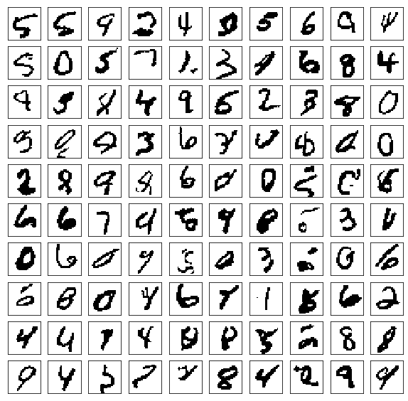
The same sampling process can use the partially occluded image as the starting point.

Now, we also try to train or model to produce an image with 256 pixel intensity.
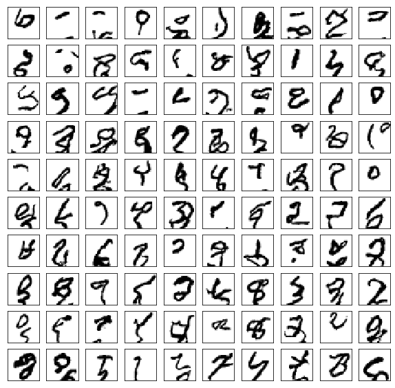
The following is an image of 256 pixel intensity with a partially occluded image as the starting point

Compared with other generation models (VAE and gan), this sampling process is relatively slow because all pixels in other models are generated at one time. However, recent research has made great progress in speed. For example, cache values can be used to reduce sampling time (such as Fast pixelcnn + +)
summary
The advantage of PixelCNN model is that joint probability learning technology is very easy to handle; we just try to predict each subsequent pixel value given all previous pixel values. Since PixelCNN is trained by minimizing negative log likelihood, it is different from other methods (such as GAN - Nash equilibrium needs to be found) Compared with its training, it is more stable, but because the sample generation is sequential (pixel by pixel), the original pixel CNN has difficulties in scalability.
quote
- http://sergeiturukin.com/2017/02/22/pixelcnn.html
- https://towardsdatascience.com/auto-regressive-generative-models-pixelrnn-pixelcnn-32d192911173
- https://deepgenerativemodels.github.io/
- https://eigenfoo.xyz/deep-autoregressive-models/
- https://wiki.math.uwaterloo.ca/statwiki/index.php?title=STAT946F17/Conditional_Image_Generation_with_PixelCNN_Decoders
- https://www.codeproject.com/Articles/5061271/PixelCNN-in-Autoregressive-Models
- https://towardsdatascience.com/blind-spot-problem-in-pixelcnn-8c71592a14a
- https://www.youtube.com/watch?v=5WoItGTWV54&t=1165s
- https://www.youtube.com/watch?v=R8fx2b8Asg0
- https://arxiv.org/pdf/1804.00779v1.pdf
- https://blog.evjang.com/2019/07/likelihood-model-tips.html
- https://arxiv.org/abs/1810.01392
- http://bjlkeng.github.io/posts/pixelcnn/
- https://jrbtaylor.github.io/conditional-pixelcnn/
- http://www.gatsby.ucl.ac.uk/~balaji/Understanding-GANs.pdf
- https://www.cs.ubc.ca/~lsigal/532S_2018W2/Lecture13b.pdf
- https://tinyclouds.org/residency/
- https://tensorflow.blog/2016/11/29/pixelcnn-1601-06759-summary/
- https://web.cs.hacettepe.edu.tr/~aykut/classes/spring2018/cmp784/slides/lec10-deep_generative_models-part-I_2.pdf
By Walter Hugo Lopez Pinaya, Pedro F. da Costa, and Jessica Dafflon