Chapter III classification
preface
In the last chapter, we learned how to complete a machine learning task, in which many models are used. In this chapter, we will have a deeper understanding of the classification model, including binary classification, multi class classification, multi label classification and multi output classification, as well as the performance measurement accuracy / recall rate and ROC of the classification model. Finally, we will use the confusion matrix to analyze the error of the model.
Let's start.
1, Mind map

2, Main content
1,MNIST
Let's briefly introduce MNIST. It is a manual handwritten picture of 7000 numbers. Each picture has 28 * 28 (784) features. The work to be completed in this chapter is to train a model to recognize numbers 0-9.
2. Training binary classifier
Let's start with a simple binary classification problem to judge whether the picture is 5 or not. The first step is the same as that mentioned in Chapter 2, loading and preliminary analysis of data.
Get and load data
It is used to get data from the Internet every time. It takes a lot of time and can't run without a network. I download the data locally and load it directly.
mnist = loadmat("./data/mnist-original.mat")
X, y = mnist["data"], mnist["label"]

# Convert the data and disrupt the order
all_data = np.vstack((X, y))
all_data = all_data.T
np.random.shuffle(all_data)
X = all_data[:, range(784)]
y = all_data[:, 784]
y = y.astype(np.uint8)
Observation and analysis of data
We mentioned earlier that this is a 28 * 28 picture. Let's take a look at what kind of digital picture it is.
# Show a picture
def show_img(data):
    """
    Show a picture
    :param data:
    :return:
    """
    data = data.reshape(28, 28)
    plt.imshow(data, cmap=mpl.cm.binary, interpolation="nearest")
    plt.axis("off")


one_digit = X[0]
plt.show()
The article also mentioned the display of multiple pictures. The specific code part is reflected in git. Here we only talk about the process.
Separate training set and test set
# Generate test and training sets
X_train, X_test, y_train, y_test = X[:60000], X[60000:], y[:60000], y[60000:]

# Train a binary classifier to distinguish between yes 5 and no 5
y_train_5 = (y_train == 5)
y_test_5 = (y_test == 5)
Training a random gradient descent two classifier
sgd_clf = SGDClassifier(random_state=42)
sgd_clf.fit(X_train, y_train_5)
print(sgd_clf.predict([one_digit]))
3. Performance measurement
Cross validation
After we have the first model, we need to verify the performance of the model. We prefer the cross validation mentioned in the previous chapter. In order to obtain higher degrees of freedom, structured kfold is used to realize custom cross validation.
# Cross validation
cvs = cross_val_score(sgd_clf, X_train, y_train_5, cv=3, scoring="accuracy")
print(cvs)

# Customize cross validation using StratifiedKFold
sk_fold = StratifiedKFold(n_splits=3, shuffle=True, random_state=42)

for train_index, test_index in sk_fold.split(X_train, y_train_5):
    clone_sgd = clone(sgd_clf)
    fold_X_train = X_train[train_index]
    fold_y_train = y_train_5[train_index]
    fold_X_test = X_train[test_index]
    fold_y_test = y_train_5[test_index]

    clone_sgd.fit(fold_X_train, fold_y_train)
    pre_y = clone_sgd.predict(fold_X_test)
    num_true = sum(np.array(fold_y_test) == np.array(pre_y))
    print(num_true / len(pre_y))
We can see that a high accuracy has been obtained. Must this accuracy be really accurate? To verify this view, we need to customize a classifier to classify all data as not 5, and then look at its accuracy.
# The purpose of customizing a classifier is to classify all data as not 5
class Never5Classifier(BaseEstimator):
    def fit(self, X, y=None):
        pass

    def predict(self, X):
        return np.zeros((len(X), 1), dtype=bool)


print(sum(y_train_5) / len(y_train_5))
print(len(X_train))
# Cross verify the performance of this all non-5 classifier
never_5 = Never5Classifier()
cvs = cross_val_score(never_5, X_train, y_train_5, cv=3, scoring="accuracy")
print(cvs)
We will find that we have also obtained an accuracy of up to 90% because the number of 5 accounts for about 10% of the total number. In order to accurately evaluate the accuracy of a classification model, we propose a good method confusion matrix.
Confusion matrix
Let's first look at the confusion matrix of the random gradient descent classifier
y_train_pred = cross_val_predict(sgd_clf, X_train, y_train_5, cv=3)
cm = confusion_matrix(y_train_5, y_train_pred)
print(cm)
Let's look at the confusion matrix of a perfect classification model
# Perfect confusion matrix
perfect_predictions = y_train_5
cm = confusion_matrix(y_train_5, perfect_predictions)
print(cm)
What is confusion matrix?
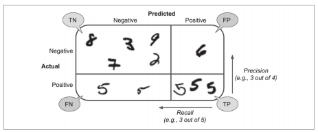
As shown in the figure, this is the confusion matrix. If it is not 5 on the upper left, it is called true negative, if it is 5 on the lower left but incorrectly classified, it is called false negative, if it is not 5 on the upper right but incorrectly classified, it is called false positive, and if it is correctly classified as 5 on the lower right, it is called true negative.
Accuracy and recall
Precision: the proportion of all instances classified as positive classes.
Recall rate: in all positive cases, the number of correctly classified accounts for.
sklearn provides two methods to calculate the two values precision_score,recall_score
# Precision and recall
precision = precision_score(y_train_5, y_train_pred)
print(precision)
recall = recall_score(y_train_5, y_train_pred)
print(recall)
In order to reflect the quality of the model with one score, sklearn provides f1 score, which combines accuracy and recall
# f1 score, a combination of precision and recall values
f1 = f1_score(y_train_5, y_train_pred)
print(f1)
Tradeoff between accuracy and recall
Many times, we will find that we can't have both fish and bear's paw. We can't guarantee a high recall rate when we obtain a high precision. At this time, we need to make a trade-off and make a balance between precision and recall rate.
We adjust the accuracy and recall by limiting the prediction threshold of the model. The cross validation model outputs the threshold value, and uses the threshold value and precision / recall rate to draw a graph to observe the process of the change of the random threshold value of precision and recall rate.
# Draw precision recall curve
y_score = cross_val_predict(sgd_clf, X_train, y_train_5, cv=3, method="decision_function")
precision, recall, threshold = precision_recall_curve(y_train_5, y_score)


def show_precision_recall_vs_threshold(precision, recall, threshold):
    """
    Displays the relationship between precision recall and threshold
    :param precision:
    :param recall:
    :param threshold:
    :return:
    """
    plt.plot(threshold, precision[:-1], "b--", label="Precision", linewidth=2)
    plt.plot(threshold, recall[:-1], "g--", label="Precision", linewidth=2)
    plt.legend(loc="center right", fontsize=16)
    plt.xlabel("Threshold", fontsize=16)
    plt.axis([-10000, 10000, 0, 1])
    plt.grid(True)


# The threshold and recall rate when the calculation accuracy reaches 90
first_max_index = np.argmax(precision >= 0.9)
precision_90_recall = recall[first_max_index]
precision_90_threshold = threshold[first_max_index]

show_precision_recall_vs_threshold(precision, recall, threshold)
# Add guides
plt.plot([precision_90_threshold, precision_90_threshold], [0., 0.9], "r:")
plt.plot([-10000, precision_90_threshold], [0.9, 0.9], "r:")
plt.plot([-10000, precision_90_threshold], [precision_90_recall, precision_90_recall], "r:")
# Add intersection
plt.plot([precision_90_threshold], [0.9], "ro")
plt.plot([precision_90_threshold], [precision_90_recall], "ro")
plt.show()
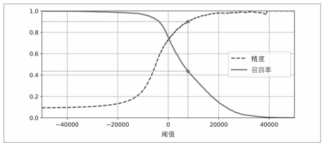
We can see that with the increase of the threshold, the accuracy also increases, but the recall rate is declining.
Now let's draw the graph of precision and recall.
def show_recall_precision(recall, precision):
    """
    Draw the relationship between recall and accuracy
    :param recall:
    :param precision:
    :return:
    """
    plt.plot(recall, precision, "b-", linewidth=2)
    plt.xlabel("Recall", fontsize=16)
    plt.ylabel("Precision", fontsize=16)
    plt.axis([0, 1, 0, 1])
    plt.grid(True)


plt.figure(figsize=(8, 6))
show_recall_precision(recall, precision)
# Calculate the recall rate when the accuracy reaches 90
precision_90_recall = recall[np.argmax(precision >= 0.9)]
# Draw guides
plt.plot([precision_90_recall, precision_90_recall], [0, 0.9], "r:")
plt.plot([0, precision_90_recall], [0.9, 0.9], "r:")
# Draw intersection
plt.plot([precision_90_recall], [0.9], "ro")
plt.show()
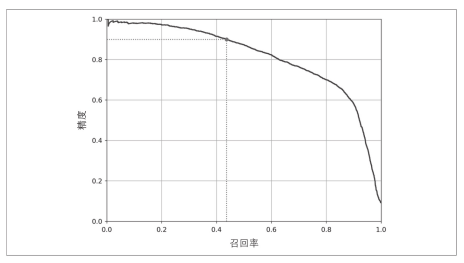
We can see that while the recall rate increases, the accuracy decreases continuously.
ROC
In addition to the precision recall rate, there is also an index to evaluate the classification model, ROC curve.
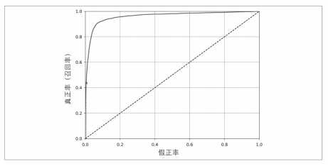
False positive rate (X-axis): it indicates the proportion of the negative category incorrectly classified in the total negative category.
True rate (Y-axis): it indicates the proportion of positive categories correctly classified in the total positive categories, and another term for recall rate.
Let's plot an ROC curve of our random gradient descent model.
# Draw roc curve
def show_roc_curve(fpr, tpr, label=None):
    plt.plot(fpr, tpr, linewidth=2, label=label)
    plt.plot([0, 1], [0, 1], "k--")
    plt.axis([0, 1, 0, 1])
    plt.xlabel("FPR", fontsize=16)
    plt.ylabel("TPR", fontsize=16)
    plt.grid(True)


plt.figure(figsize=(8, 6))
show_roc_curve(fpr, tpr)
# Check the value of fpr when the recall rate (tpr) reaches 90
fpr_precision_90 = fpr[np.argmax(tpr >= precision_90_recall)]
print(fpr_precision_90)
plt.plot([fpr_precision_90, fpr_precision_90], [0, precision_90_recall], ":r")
plt.plot([0, fpr_precision_90], [precision_90_recall, precision_90_recall], ":r")
plt.plot([fpr_precision_90], [precision_90_recall], "ro")
plt.show()
Another expression of ROC curve is AUC, which is the area of ROC curve. The closer AUC is to 1, the more accurate the model is.
# View auc of roc curve
auc = roc_auc_score(y_train_5, y_score)
print(auc)
Next, we train a random forest model, and then compare the ROC curves of the two models.
# Training a random forest classifier model
forest_fcl = RandomForestClassifier(n_estimators=100, random_state=42)
forest_fcl.fit(X_train, y_train_5)
# Cross validation
y_proba_forest = cross_val_predict(forest_fcl, X_train, y_train_5, cv=3, method="predict_proba")
y_score_forest = y_proba_forest[:, 1]

# Draw roc curve
fpr_forest, tpr_forest, thresholds_forest = roc_curve(y_train_5, y_score_forest)
tpr_forest_90 = tpr_forest[np.argmax(fpr_forest >= fpr_precision_90)]

plt.figure(figsize=(8, 6))
plt.plot(fpr_forest, tpr_forest, label="RANDOM FOREST")
show_roc_curve(fpr, tpr, label="SGD")
# Draw guides
plt.plot([fpr_precision_90, fpr_precision_90], [0., precision_90_recall], "r:")
plt.plot([0., fpr_precision_90], [precision_90_recall, precision_90_recall], "r:")
plt.plot([fpr_precision_90, fpr_precision_90], [0., tpr_forest_90], "r:")
plt.plot([fpr_precision_90], [precision_90_recall], "ro")
plt.plot([fpr_precision_90], [tpr_forest_90], "ro")
plt.legend(loc="lower right", fontsize=16)
plt.grid(True)
plt.axis([0, 1, 0, 1])
plt.show()
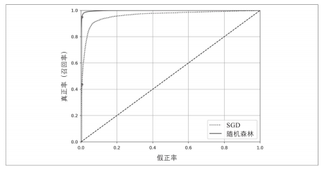
From the figure, we can see that the area of random forest model is larger than that of SGD, and the curve is closer to the upper left corner, indicating that the performance of random forest model is better than that of SGD. Let's look at the precision recall and AUC of the random forest model
# Calculate auc, recall and accuracy
auc = roc_auc_score(y_train_5, y_score_forest)
print(auc)

predict_forest = cross_val_predict(forest_fcl, X_train, y_train_5, cv=3)
print(predict_forest)
recall_forest = recall_score(y_train_5, predict_forest)
print(recall_forest)

precision_forest = precision_score(y_train_5, predict_forest)
print(precision_forest)
4. Multiclass classifier
We have completed the training of binary classifier. The model can only predict whether it is 5 or not, which can not meet our expectations. We need to identify all numbers 0-9. So now we need to train a multi class classifier SVC.
svm_clf = SVC(gamma="auto", random_state=42)
svm_clf.fit(X[:1000], y_train[:1000])
svm_predict = svm_clf.predict([one_digit])
# print(svm_predict)

svm_dec = svm_clf.decision_function([one_digit])
print(svm_dec)

print(svm_clf.classes_)

print(svm_clf.classes_[7])
For multi class classifiers, we generally have two strategies to complete one-to-one (5 or other) and one-to-one (5 or 3). For models with small data sets, we can use one-to-one strategy. Under normal circumstances, we will still use one-to-one strategy.
We use SGDClassifier, support vector (SVC) and random forest classifier to train a pair of remaining models to complete the prediction.
# Train a pair of residual models
ovr_clf = OneVsRestClassifier(SVC(gamma="auto", random_state=42))
ovr_clf.fit(X[:1000], y_train[:1000])
ovr_predict = ovr_clf.predict([one_digit])
print(ovr_predict)

sgd_clf = SGDClassifier(random_state=42)
sgd_clf.fit(X[:1000], y_train[:1000])
sgd_predict = sgd_clf.predict([one_digit])
print(sgd_predict)

random_forest_clf = RandomForestClassifier(random_state=42)
random_forest_clf.fit(X[:1000], y_train[:1000])
random_forest_predict = random_forest_clf.predict([one_digit])
print(random_forest_predict)
Here we mention a small knowledge point and use normalization to improve the accuracy of the model.
# Verify whether normalization can improve accuracy
sgd_score = cross_val_score(sgd_clf, X_train, y_train, cv=3, scoring="accuracy")
print(sgd_score)
scaler = StandardScaler()
X_train_scaled = scaler.fit_transform(X_train.astype(np.float64))
sgd_scaled_score = cross_val_score(sgd_clf, X_train_scaled, y_train, cv=3)
print(sgd_scaled_score)
5. Error analysis
After obtaining a multi class classification, we need to continue to use confusion proof to analyze the error of the model. First, we will generate a confusion proof manually, and then draw the confusion matrix with the method provided by sklearn.
sgd_clf = SGDClassifier(random_state=42)
y_train_predict = cross_val_predict(sgd_clf, X_train, y_train, cv=3)
sgd_cm = confusion_matrix(y_train, y_train_predict)

def show_confusion_matrix(matrix):
    """
    Draw confusion matrix manually
    :param matrix:
    :return:
    """
    fig = plt.figure(figsize=(8, 6))
    ax = fig.add_subplot(111)
    cax = ax.matshow(matrix)
    fig.colorbar(cax)


show_confusion_matrix(sdg_cm)
plt.show()

# Draw confusion matrix with sklearn
plt.matshow(sgd_cm, cmap=plt.cm.gray)
plt.show()
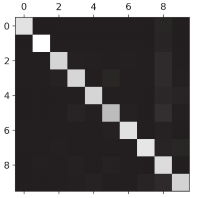
The confusion matrix drawn seems to be OK to the naked eye without too much error. That's because the number of 0-9 in all 70000 pictures is not evenly distributed. We need to multiply the value of the confusion matrix by the proportion of the number and draw the confusion matrix again.
# Calculate the number of pictures for each category
row_nums = sgd_cm.sum(axis=1, keepdims=True)
# Considering that the number of pictures of each number is different, considering the accuracy of the data, we need to divide the value of the confusion matrix by its number
norm_sgd_cm = sgd_cm / row_nums
# Fill diagonal with 0
np.fill_diagonal(norm_sgd_cm, 0)
plt.matshow(norm_sgd_cm, cmap=plt.cm.gray)
plt.show()
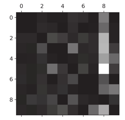
You can see that the color of the 8 column is white, so it means that there are more books predicted to be classified as 8, of which 5 is the most.
It is not clear why the book does not continue to display the pictures of 8 and 5, but chooses to display the classification of 5 and 3.
# Check for confusion between 3 and 5
num_3, num_5 = 3, 5
X_33 = X_train[(y_train == num_3) & (y_train_predict == num_3)]
X_35 = X_train[(y_train == num_3) & (y_train_predict == num_5)]
X_53 = X_train[(y_train == num_5) & (y_train_predict == num_3)]
X_55 = X_train[(y_train == num_5) & (y_train_predict == num_5)]

# Draw the error classification diagram of 3 and 5. The upper left corner is correctly classified as 3 and the upper right corner is incorrectly classified as 3
# The lower left corner is the picture of 3 incorrectly classified as 5, and the lower right corner is the picture correctly classified as 5
plt.figure(figsize=(8, 8))
plt.subplot(221)
show_digit(X_33[:25], num_per_row=5)
plt.subplot(222)
show_digit(X_35[:25], num_per_row=5)
plt.subplot(223)
show_digit(X_53[:25], num_per_row=5)
plt.subplot(224)
show_digit(X_55[:25], num_per_row=5)
plt.show()
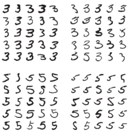
We can see that there are many pictures that we can't distinguish ourselves, which is the reason why our model prediction is wrong.
6. Multi label classification
What we have done before is to predict one instance and one label. Now we need to upgrade the difficulty. We need to classify multiple labels at the same time, whether a number is odd or greater than 7.
A K-nearest neighbor algorithm is trained to complete this task, because not all classifiers support multi label classification.
# Multi label classification
y_train_large = (y_train >= 7)
y_train_even = (y_train % 2 == 0)
y_train_large_odd = np.c_[y_train_large, y_train_even]
# Training model using K-nearest neighbor algorithm
knn_clf = KNeighborsClassifier()
knn_clf.fit(X_train, y_train_large_odd)
knn_predict = knn_clf.predict([one_digit])
print(knn_predict)
7. Multiple output classification
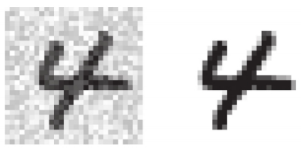
Again, we need more output to complete the noise reduction function of a picture.
Add noise
Finish adding noise and view the finished picture.
# Add noise to pictures
noise = np.random.randint(0, 100, (len(X_train), 784))
X_train_noise = X_train + noise
noise = np.random.randint(0, 100, (len(X_test), 784))
X_test_noise = X_test + noise
y_train_noise = X_train


# Displays the difference between adding noise and not adding noise
plt.figure(figsize=(8, 4))
plt.subplot(121)
show_img(X_test[0])
plt.subplot(122)
show_img(X_test_noise[0])
plt.show()
Training model
knn_clf = KNeighborsClassifier()
knn_clf.fit(X_train_noise, y_train_noise)
clean_digit = knn_clf.predict([X_test_noise[0]])
show_img(clean_digit)
plt.show()
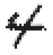
As shown in the figure, this is the picture after noise reduction.
3, After class practice
1. Build a classifier for MNIST data set and achieve an accuracy of more than 97% on the test set. Tip: kneigborsclassifier is very effective for this task. You only need to find the appropriate hyperparameter value (try grid search for the two hyperparameters weights and n_neighbors).
# Build mesh parameters
grid_param = [{"weights": ["uniform", "distance"], "n_neighbors": [3, 4, 5]}]
# Start grid search
knn_clf = KNeighborsClassifier()
grid_cv = GridSearchCV(knn_clf, grid_param, cv=5, verbose=3)
grid_cv.fit(X_train, y_train)

print(grid_cv.best_estimator_)
print(grid_cv.best_score_)
knn_test_predict = grid_cv.predict(X_test)
knn_score = accuracy_score(y_test, knn_test_predict)
print(knn_score)
2. Write a function that can move MNIST pictures by one pixel in any direction (up, down, left and right) [1]. Then create four displaced copies of each picture in the training set (one in each direction) is added to the training set. Finally, train the model on this extended training set and measure its accuracy on the test set. You should notice that the performance of the model has even become better! This technology of manually expanding the training set is called data augmentation or training set expansion.
# Set picture offset
def shift_image(image, dx, dy):
    image = image.reshape(28, 28)
    shifted_image = shift(image, [dx, dy], cval=0)
    return shifted_image.reshape([-1])

shifted_image_down = shift_image(one_digit, -5, 0)
plt.figure(figsize=(8, 4))
plt.subplot(121)
plt.title("Original", fontsize=16)
plt.imshow(one_digit.reshape(28, 28), interpolation="nearest", cmap="Greys")
plt.subplot(122)
plt.title("Shift", fontsize=16)
plt.imshow(shifted_image_down.reshape(28, 28), interpolation="nearest", cmap="Greys")
plt.show()

# Circular offset picture
X_train_augmented = [image for image in X_train]
y_train_augmented = [image for image in y_train]

for dx, dy in [(1, 0), (-1, 0), (0, 1), (0, -1)]:
    for image, label in zip(X_train, y_train):
        X_train_augmented.append(shift_image(image, dx, dy))
        y_train_augmented.append(label)

X_train_augmented = np.array(X_train_augmented)
y_train_augmented = np.array(y_train_augmented)

# Disorder order
per_index = np.random.permutation(len(X_train_augmented))
X_train_augmented = X_train_augmented[per_index]
y_train_augmented = y_train_augmented[per_index]

# Training model
knn_clf = KNeighborsClassifier(n_neighbors=4, weights='distance')
knn_clf.fit(X_train_augmented, y_train_augmented)
knn_augmented_predict = knn_clf.predict(X_test)
knn_augmented_score = accuracy_score(y_test, knn_augmented_predict)
print(knn_augmented_score)
3. A great starting point on kaggle: processing the Titanic dataset.
Titanic article address
4. Create a spam classifier (more challenging exercise)
Because there are many codes here, I put all the codes in git.
4, Summary
In this chapter, we completed the classification of MNIST, from binary classifier to multi class classifier and multi label classifier... Step by step, and finally completed the classification of 0-9 numbers. While completing the classification, we also mentioned a key point, the performance measurement of the classification model. It is divided into two key points: 1. Accuracy and recall rate; 2. ROC.
Friends who have any doubts about the article or want to learn machine learning with bloggers can add the group number: 666980220. If you need machine learning, actual combat electronic version or mind map, you can also contact me. Good luck!
Project address: github