For more documentation on Apache ECharts, please read:
Apache ECharts tutorial
- Get started in 5 minutes, ECharts
- What's new in ECharts 5
- ECharts 5 upgrade Guide
- Using ECharts in a packaged environment
- Overview of basic concepts of ECharts
- Style of personalized chart
- Introduction to styles in ECharts
- Asynchronous data loading and updating
- Managing data using dataset s
- Data conversion using transform part I
- Data conversion using transform part II
- Add interactive components to the diagram
- Mobile terminal adaptation
- Visual mapping of data
- Events and behaviors in ECharts
- Dynamic sorting histogram
- Small example: drag and drop by yourself
- Small example: implement calendar chart
- Rising sun chart
- Custom series
- Rich text label
- Server side rendering
- Render using Canvas or SVG
- SVG basemap of geographic coordinate system and map series
- Support accessibility in charts
- Basic 3D visualization using ecarts GL
- Using ecarts in wechat applet
Ecarts GL (hereinafter referred to as GL) adds rich 3D visualization components to Apache ecartstm. In this article, we will briefly introduce how to realize some common 3D visualization works based on GL. In fact, if you have a certain understanding of ECharts, you can also get started with GL quickly. The configuration items of GL are designed completely according to the standards and difficulty of ECharts.
After reading the article, you can go to the official examples and Gallery to learn more examples made with GL. For the codes we can't explain in the article, you can also go to the GL configuration item manual to see the specific usage methods of configuration items.
How to download and import ECharts GL
In order not to increase the volume of the full version of ecarts, which is already very large, we provide GL as an extension package. Similar to extensions such as water polo diagram, if you want to use various components in GL, you only need to introduce ecarts Min. JS, and then an ECharts GL min.js. You can download the latest version of GL from the official website, and then introduce it in the page through the label:
<script src="lib/echarts.min.js"></script>
<script src="lib/echarts-gl.min.js"></script>
If your project uses webpack or rollup to package code, it can also be imported after npm installation
npm install echarts
npm install echarts-gl
// ECharts and ECharts GL are introduced through the import syntax of ES6
import echarts from 'echarts';
import 'echarts-gl';
Declare a basic three-dimensional Cartesian coordinate system
After introducing ECharts and ECharts GL, we first declare a basic three-dimensional Cartesian coordinate system for drawing three-dimensional scatter diagrams, histogram, surface diagrams and other common statistical diagrams.
In ECharts, we have a grid component to provide a rectangular area to place a two-dimensional Cartesian coordinate system and the x-axis and y-axis on the Cartesian coordinate system. For the three-dimensional Cartesian coordinate system, we provide the grid3D component in GL to divide a three-dimensional Cartesian space and the xAxis3d, yAxis3d and zaxis3d placed on the grid3D.
Tip: in GL, we add 3D suffix to all 3D components and series except globe to distinguish them. For example, 3D scatter map is scatter3D, 3D map is map3D, etc.
The following code declares the simplest three-dimensional Cartesian coordinate system
var option = {
    // It should be noted that we cannot omit grid3D like grid
    grid3D: {},
    // By default, x, y, and Z are numerical axes from 0 to 1, respectively
    xAxis3D: {},
    yAxis3D: {},
    zAxis3D: {}
}
The effects are as follows:
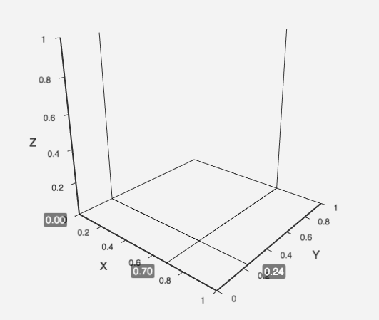
Like the two-dimensional Cartesian coordinate system, each axis has multiple types. The default is the numerical axis. If it needs to be the category axis, simply set it to type: 'category'.
Draw a three-dimensional scatter diagram
After declaring the Cartesian coordinate system, we first try to draw a scatter diagram in this three-dimensional Cartesian coordinate system with the normal distribution data generated by a program.
The following section is the code for generating normal distribution data. You don't need to care about how this code works first. You just need to know that it generates a three-dimensional normal distribution data and puts it in the data array.
function makeGaussian(amplitude, x0, y0, sigmaX, sigmaY) {
    return function (amplitude, x0, y0, sigmaX, sigmaY, x, y) {
        var exponent = -(
                ( Math.pow(x - x0, 2) / (2 * Math.pow(sigmaX, 2)))
                + ( Math.pow(y - y0, 2) / (2 * Math.pow(sigmaY, 2)))
            );
        return amplitude * Math.pow(Math.E, exponent);
    }.bind(null, amplitude, x0, y0, sigmaX, sigmaY);
}
// Create a Gaussian distribution function
var gaussian = makeGaussian(50, 0, 0, 20, 20);

var data = [];
for (var i = 0; i < 1000; i++) {
    // x. Y random distribution
    var x = Math.random() * 100 - 50;
    var y = Math.random() * 100 - 50;
    var z = gaussian(x, y);
    data.push([x, y, z]);
}
The generated normally distributed data is approximately as follows:
[
  [46.74395071259907, -33.88391024738553, 0.7754030099768191],
  [-18.45302873809771, 16.88114775416834, 22.87772504105404],
  [2.9908128281121336, -0.027699444453467947, 49.44400635911886],
  ...
]
Each term contains three values of x, y and z, which are mapped to the x, y and z axes of the Cartesian coordinate system.
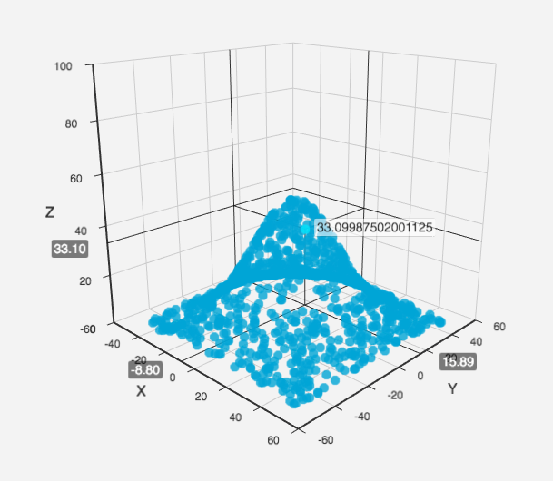
Then we can use the scatter3D series type provided by GL to draw these data into normally distributed points in three-dimensional space.
option = {
    grid3D: {},
    xAxis3D: {},
    yAxis3D: {},
    zAxis3D: { max: 100 },
    series: [{
        type: 'scatter3D',
        data: data
    }]
}
3D scatter plot using real data
Next, let's look at an example of a 3D scatter diagram using real multidimensional data.
You can start with https://echarts.apache.org/examples/data/asset/data/life-expectancy-table.json Get this data.
After formatting, you can see that this data is a very traditional table format after being converted to JSON. The first row is the attribute name of each column of data. You can see the meaning of each column of data from this attribute name, including per capita income, per capita life expectancy, population, country and year.
[
    ["Income", "Life Expectancy", "Population", "Country", "Year"],
    [815, 34.05, 351014, "Australia", 1800],
    [1314, 39, 645526, "Canada", 1800],
    [985, 32, 321675013, "China", 1800],
    [864, 32.2, 345043, "Cuba", 1800],
    [1244, 36.5731262, 977662, "Finland", 1800],
    ...
]
In ECharts 4, we can use the dataset component to easily import this data. If you are not familiar with dataset, you can see the dataset tutorial
$.get('data/asset/data/life-expectancy-table.json', function (data) {
    myChart.setOption({
        grid3D: {},
        xAxis3D: {},
        yAxis3D: {},
        zAxis3D: {},
        dataset: {
            source: data
        },
        series: [
            {
                type: 'scatter3D',
                symbolSize: 2.5
            }
        ]
    })
});
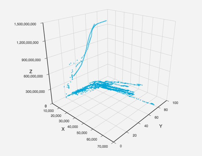
By default, the first three columns, namely Income, Life Expectancy and Population, will be placed on the x, y and z axes respectively.
Using the encode attribute, we can also map the data of the specified column to the specified coordinate axis, so as to save a lot of cumbersome data conversion code. For example, if we change the x-axis to Country, the y-axis to Year, and the z-axis to Income, we can see the distribution of per capita Income in different countries in different years.
myChart.setOption({
    grid3D: {},
    xAxis3D: {
        // Because both x-axis and y-axis are category data, you need to set type: 'category' to ensure correct data display.
        type: 'category'
    },
    yAxis3D: {
        type: 'category'
    },
    zAxis3D: {},
    dataset: {
        source: data
    },
    series: [
        {
            type: 'scatter3D',
            symbolSize: 2.5,
            encode: {
                // The name of the dimension is the attribute name of the header by default
                x: 'Country',
                y: 'Year',
                z: 'Income',
                tooltip: [0, 1, 2, 3, 4]
            }
        }
    ]
});
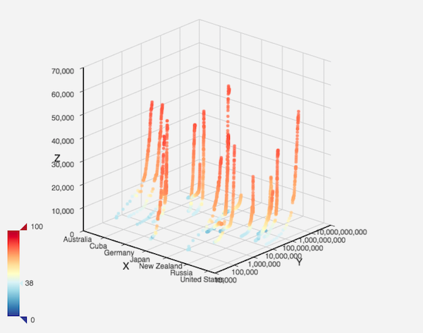
Visual coding of 3D scatter diagram using visual map component
In the example of multidimensional data just now, we still have several dimensions (columns) that can not be expressed. Using the built-in visual map component of ECharts, we can continue to encode the fourth dimension into color.
myChart.setOption({
    grid3D: {
        viewControl: {
            // Use orthogonal projection.
            projection: 'orthographic'
        }
    },
    xAxis3D: {
        // Because both x-axis and y-axis are category data, you need to set type: 'category' to ensure correct data display.
        type: 'category'
    },
    yAxis3D: {
        type: 'log'
    },
    zAxis3D: {},
    visualMap: {
        calculable: true,
        max: 100,
        // The name of the dimension is the attribute name of the header by default
        dimension: 'Life Expectancy',
        inRange: {
            color: ['#313695', '#4575b4', '#74add1', '#abd9e9', '#e0f3f8', '#ffffbf', '#fee090', '#fdae61', '#f46d43', '#d73027', '#a50026']
        }
    },
    dataset: {
        source: data
    },
    series: [
        {
            type: 'scatter3D',
            symbolSize: 5,
            encode: {
                // The name of the dimension is the attribute name of the header by default
                x: 'Country',
                y: 'Population',
                z: 'Income',
                tooltip: [0, 1, 2, 3, 4]
            }
        }
    ]
})
In this code, we added the visual map component based on the example just now to map the data in the column of life expectation to different colors.
In addition, we also changed the original default perspective projection to orthogonal projection. Orthogonal projection can avoid the expression error caused by near large and far small in some scenes.
Of course, in addition to the visual map component, you can also use other built-in components of ECharts and make full use of the interaction effects of these components, such as legend. You can also realize the mixing of two-dimensional and three-dimensional series like the combination of three-dimensional scatter diagram and scatter matrix.
When implementing GL, we try to minimize the difference between WebGL and Canvas, so that the use of GL can be more convenient and natural.
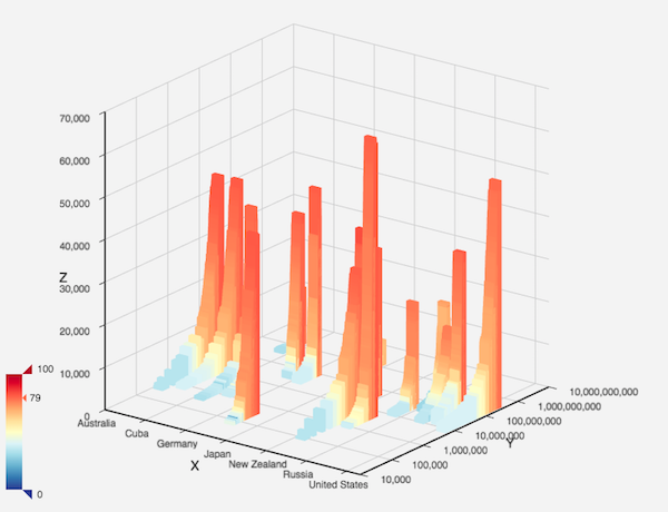
Display other types of 3D charts in Cartesian coordinate system
In addition to scatter charts, we can also draw other types of three-dimensional charts on the three-dimensional Cartesian coordinate system through GL. For example, in the example just now, changing the scatter3D type to bar3D can turn into a three-dimensional histogram.
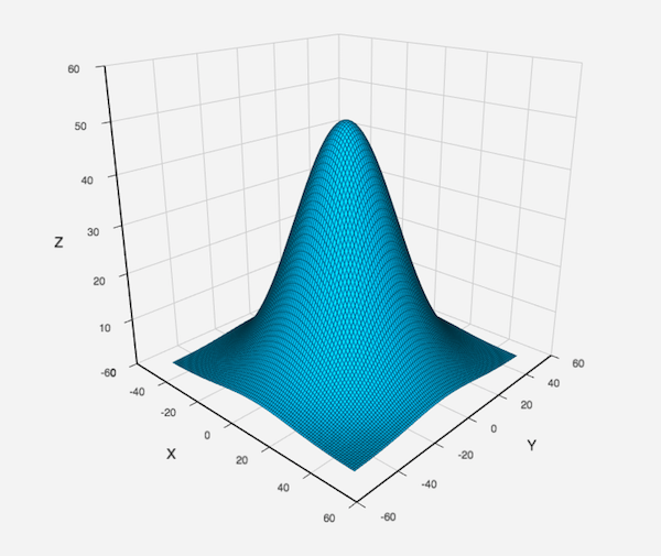
There is also the three-dimensional surface graph used in machine learning. The three-dimensional surface graph is often used to express the data trend on the plane. We can also draw the normal distribution data as follows.
var data = [];
// Surface graph requires that the data given in is in the form of grid and distributed in order.
for (var y = -50; y <= 50; y++) {
    for (var x = -50; x <= 50; x++) {
        var z = gaussian(x, y);
        data.push([x, y, z]);
    }
}
option = {
    grid3D: {},
    xAxis3D: {},
    yAxis3D: {},
    zAxis3D: { max: 60 },
    series: [{
        type: 'surface',
        data: data
    }]
}
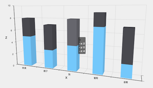
The boss wants a three-dimensional histogram effect
Finally, we are often asked how to draw a three-dimensional histogram with only two-dimensional data with ECharts. Generally speaking, we do not recommend this, because this unnecessary three-dimensional histogram is easy to cause wrong expression. For details, see the explanation in our histogram use guide.
However, if some other factors lead to the need to draw a three-dimensional histogram, it can also be achieved with GL. Similar examples have been written in the Gallery for you to refer to.
3D stacked histogram
3D histogram