import numpy as np
import mxnet as mx
import logging
logging.getLogger().setLevel(logging.DEBUG)  # logging to stdout
mxnet basic data structure
ndarray
Ndarray is the most basic data structure in mxnet. The relationship between ndarray and mxnet is similar to that between tensor and pytorch.This data structure can be seen as a variant of numpy, and basically numpy's operation ndarray can be implemented.The ndarray-related section is mxnet.nd., and the API for the ndarray operation can be viewed officially API Documentation
ndarray operation
a = mx.nd.random.normal(shape=(4,3))
b = mx.nd.ones((4,3))
print(a)
print(b)
print(a + b)
[[ 0.23107234  0.30030754 -0.32433936]
 [ 1.04932904  0.7368623  -0.0097888 ]
 [ 0.46656415  1.72023427  0.87809837]
 [-1.07333779 -0.86925656 -0.26717702]]
<NDArray 4x3 @cpu(0)>

[[ 1.  1.  1.]
 [ 1.  1.  1.]
 [ 1.  1.  1.]
 [ 1.  1.  1.]]
<NDArray 4x3 @cpu(0)>

[[ 1.23107231  1.30030751  0.67566061]
 [ 2.04932904  1.7368623   0.99021119]
 [ 1.46656418  2.72023439  1.87809837]
 [-0.07333779  0.13074344  0.73282301]]
<NDArray 4x3 @cpu(0)>
ndarray and numpy convert to each other
- mxnet.nd.array() can be converted to nd array by passing in a numpy matrix
- Using the ndarray.asnumpy() method to convert ndarray to a numpy matrix
a = np.random.randn(2,3)
print(a,type(a))
b = mx.nd.array(a)
print(b,type(b))
b = b.asnumpy()
print(b,type(b))
[[ 0.85512384 -0.58311797 -1.41627038]
 [-0.56862628  1.15431958  0.13168715]] <class 'numpy.ndarray'>

[[ 0.85512382 -0.58311796 -1.41627038]
 [-0.56862628  1.15431952  0.13168715]]
<NDArray 2x3 @cpu(0)> <class 'mxnet.ndarray.ndarray.NDArray'>
[[ 0.85512382 -0.58311796 -1.41627038]
 [-0.56862628  1.15431952  0.13168715]] <class 'numpy.ndarray'>
symbol
Symbol is another important concept that can be understood as a symbol, just like the algebraic symbols x, y, z that we usually use.A simple analogy is a function of $f(x) = x^{2}$, the symbol x is the symbol, and the value of the specific x is ndarray, the symbols are mxnet.sym., referring to the official API Documentation
basic operation
- Create a symbol using the mxnet.sym.Variable() incoming name
- Operational diagrams can be drawn using the mxnet.viz.plot_network(symbol=) incoming symbols
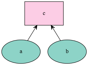
a = mx.sym.Variable('a')
b = mx.sym.Variable('b')
c = mx.sym.add_n(a,b,name="c")
mx.viz.plot_network(symbol=c)
Bring in ndarray
Using the mxnet.sym.bind() method, you can get an object with an operand, and then use the forward() method to calculate the value.
x = c.bind(ctx=mx.cpu(),args={"a": mx.nd.ones(5),"b":mx.nd.ones(5)})
result = x.forward()
print(result)
[
[ 2.  2.  2.  2.  2.]
<NDArray 5 @cpu(0)>]
Data loading for mxnet
The way data is loaded is very important for in-depth learning. mxnet provides a series of dataiter s for mxnet.io. to handle data loading, which can be referred to in detail Official API Documentation .The dynamic graph interface gluon also provides a dataiter of the mxnet.gluon.data.series for data loading, which can be referred to in detail. Official API Documentation
mxnet.io data loading
The core of data loading for mxnet.io is the mxnet.io.DataIter class and its derived classes, such as iter:NDArrayIter for ndarray
- Parameter data=: Data dict passed in (name-data)
- Parameter label=: passed in a label dict (name-label)
- Parameter batch_size=: Incoming batch size
dataset = mx.io.NDArrayIter(data={'data':mx.nd.ones((10,5))},label={'label':mx.nd.arange(10)},batch_size=5)
for i in dataset:
    print(i)
    print(i.data,type(i.data[0]))
    print(i.label,type(i.label[0]))
DataBatch: data shapes: [(5, 5)] label shapes: [(5,)]
[
[[ 1.  1.  1.  1.  1.]
 [ 1.  1.  1.  1.  1.]
 [ 1.  1.  1.  1.  1.]
 [ 1.  1.  1.  1.  1.]
 [ 1.  1.  1.  1.  1.]]
<NDArray 5x5 @cpu(0)>] <class 'mxnet.ndarray.ndarray.NDArray'>
[
[ 0.  1.  2.  3.  4.]
<NDArray 5 @cpu(0)>] <class 'mxnet.ndarray.ndarray.NDArray'>
DataBatch: data shapes: [(5, 5)] label shapes: [(5,)]
[
[[ 1.  1.  1.  1.  1.]
 [ 1.  1.  1.  1.  1.]
 [ 1.  1.  1.  1.  1.]
 [ 1.  1.  1.  1.  1.]
 [ 1.  1.  1.  1.  1.]]
<NDArray 5x5 @cpu(0)>] <class 'mxnet.ndarray.ndarray.NDArray'>
[
[ 5.  6.  7.  8.  9.]
<NDArray 5 @cpu(0)>] <class 'mxnet.ndarray.ndarray.NDArray'>
gluon.data data data data loading
gluon's data API is almost identical to pytorch's, both in the way of Dataset+DataLoader:
- Dataset: Stores data and inherits the base class when used and overloads the u len_u (self) and u getitem_ (self, idx) methods
- DataLoader: Turn a Dataset into an iterative object that generates batch es
dataset = mx.gluon.data.ArrayDataset(mx.nd.ones((10,5)),mx.nd.arange(10))
loader = mx.gluon.data.DataLoader(dataset,batch_size=5)
for i,data in enumerate(loader):
    print(i)
    print(data)
0
[
[[ 1.  1.  1.  1.  1.]
 [ 1.  1.  1.  1.  1.]
 [ 1.  1.  1.  1.  1.]
 [ 1.  1.  1.  1.  1.]
 [ 1.  1.  1.  1.  1.]]
<NDArray 5x5 @cpu(0)>,
[ 0.  1.  2.  3.  4.]
<NDArray 5 @cpu(0)>]
1
[
[[ 1.  1.  1.  1.  1.]
 [ 1.  1.  1.  1.  1.]
 [ 1.  1.  1.  1.  1.]
 [ 1.  1.  1.  1.  1.]
 [ 1.  1.  1.  1.  1.]]
<NDArray 5x5 @cpu(0)>,
[ 5.  6.  7.  8.  9.]
<NDArray 5 @cpu(0)>]
class TestSet(mx.gluon.data.Dataset):
    def __init__(self):
        self.x = mx.nd.zeros((10,5))
        self.y = mx.nd.arange(10)

    def __getitem__(self,i):
        return self.x[i],self.y[i]

    def __len__(self):
        return 10

for i,data in enumerate(mx.gluon.data.DataLoader(TestSet(),batch_size=5)):
    print(data)
[
[[ 0.  0.  0.  0.  0.]
 [ 0.  0.  0.  0.  0.]
 [ 0.  0.  0.  0.  0.]
 [ 0.  0.  0.  0.  0.]
 [ 0.  0.  0.  0.  0.]]
<NDArray 5x5 @cpu(0)>,
[[ 0.]
 [ 1.]
 [ 2.]
 [ 3.]
 [ 4.]]
<NDArray 5x1 @cpu(0)>]
[
[[ 0.  0.  0.  0.  0.]
 [ 0.  0.  0.  0.  0.]
 [ 0.  0.  0.  0.  0.]
 [ 0.  0.  0.  0.  0.]
 [ 0.  0.  0.  0.  0.]]
<NDArray 5x5 @cpu(0)>,
[[ 5.]
 [ 6.]
 [ 7.]
 [ 8.]
 [ 9.]]
<NDArray 5x1 @cpu(0)>]
Network Setup
mxnet network building
The mxnet network is built like TensorFlow, using symbol s to build the network, and encapsulated in a module
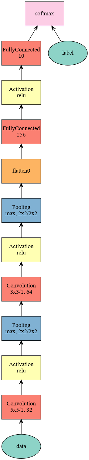
data = mx.sym.Variable('data')
# layer1
conv1 = mx.sym.Convolution(data=data, kernel=(5,5), num_filter=32,name="conv1")
relu1 = mx.sym.Activation(data=conv1,act_type="relu",name="relu1")
pool1 = mx.sym.Pooling(data=relu1,pool_type="max",kernel=(2,2),stride=(2,2),name="pool1")

# layer2
conv2 = mx.sym.Convolution(data=pool1, kernel=(3,3), num_filter=64,name="conv2")
relu2 = mx.sym.Activation(data=conv2,act_type="relu",name="relu2")
pool2 = mx.sym.Pooling(data=relu2,pool_type="max",kernel=(2,2),stride=(2,2),name="pool2")

# layer3
fc1 = mx.symbol.FullyConnected(data=mx.sym.flatten(pool2), num_hidden=256,name="fc1")
relu3 = mx.sym.Activation(data=fc1, act_type="relu",name="relu3")

# layer4
fc2 = mx.symbol.FullyConnected(data=relu3, num_hidden=10,name="fc2")
out = mx.sym.SoftmaxOutput(data=fc2, label=mx.sym.Variable("label"),name='softmax')

mxnet_model = mx.mod.Module(symbol=out,label_names=["label"],context=mx.gpu())
mx.viz.plot_network(symbol=out)
Gluon Model Building
Gluon model building is similar to pytorch by inheriting an mx.gluon.Block or using mx.gluon.nn.Sequential()
General construction method
class MLP(mx.gluon.Block):
    def __init__(self, **kwargs):
        super(MLP, self).__init__(**kwargs)
        with self.name_scope():
            self.dense0 = mx.gluon.nn.Dense(256)
            self.dense1 = mx.gluon.nn.Dense(64)
            self.dense2 = mx.gluon.nn.Dense(10)

    def forward(self, x):
        x = mx.nd.relu(self.dense0(x))
        x = mx.nd.relu(self.dense1(x))
        x = self.dense2(x)
        return x
gluon_model = MLP()
print(gluon_model)
# mx.viz.plot_network(symbol=gluon_model)
MLP(
  (dense0): Dense(None -> 256, linear)
  (dense2): Dense(None -> 10, linear)
  (dense1): Dense(None -> 64, linear)
)
Quick build method
gluon_model2 = mx.gluon.nn.Sequential()
with gluon_model2.name_scope():
    gluon_model2.add(mx.gluon.nn.Dense(256,activation="relu"))
    gluon_model2.add(mx.gluon.nn.Dense(64,activation="relu"))
    gluon_model2.add(mx.gluon.nn.Dense(10,activation="relu"))
print(gluon_model2)
Sequential(
  (0): Dense(None -> 256, Activation(relu))
  (1): Dense(None -> 64, Activation(relu))
  (2): Dense(None -> 10, Activation(relu))
)
model training
mxnet model training
mxnet provides two different levels of training encapsulation, generally using the most convenient top-level encapsulation fit()
mnist = mx.test_utils.get_mnist()
train_iter = mx.io.NDArrayIter(mnist['train_data'], mnist['train_label'], batch_size=100, data_name='data',label_name='label',shuffle=True)
val_iter = mx.io.NDArrayIter(mnist['test_data'], mnist['test_label'], batch_size=100,data_name='data',label_name='label')
INFO:root:train-labels-idx1-ubyte.gz exists, skipping download
INFO:root:train-images-idx3-ubyte.gz exists, skipping download
INFO:root:t10k-labels-idx1-ubyte.gz exists, skipping download
INFO:root:t10k-images-idx3-ubyte.gz exists, skipping download
mxnet_model.fit(train_iter,  # train data
              eval_data=val_iter,  # validation data
              optimizer='adam',  # use SGD to train
              optimizer_params={'learning_rate':0.01},  # use fixed learning rate
              eval_metric='acc',  # report accuracy during training
              batch_end_callback = mx.callback.Speedometer(100, 200), # output progress for each 100 data batches
              num_epoch=3)  # train for at most 3 dataset passes
INFO:root:Epoch[0] Batch [200]  Speed: 5239.83 samples/sec  accuracy=0.890348
INFO:root:Epoch[0] Batch [400]  Speed: 5135.49 samples/sec  accuracy=0.971450
INFO:root:Epoch[0] Train-accuracy=0.977236
INFO:root:Epoch[0] Time cost=11.520
INFO:root:Epoch[0] Validation-accuracy=0.980300
INFO:root:Epoch[1] Batch [200]  Speed: 5336.36 samples/sec  accuracy=0.979453
INFO:root:Epoch[1] Batch [400]  Speed: 5312.22 samples/sec  accuracy=0.982550
INFO:root:Epoch[1] Train-accuracy=0.984724
INFO:root:Epoch[1] Time cost=11.704
INFO:root:Epoch[1] Validation-accuracy=0.980500
INFO:root:Epoch[2] Batch [200]  Speed: 5522.89 samples/sec  accuracy=0.982388
INFO:root:Epoch[2] Batch [400]  Speed: 5562.08 samples/sec  accuracy=0.984550
INFO:root:Epoch[2] Train-accuracy=0.985075
INFO:root:Epoch[2] Time cost=10.860
INFO:root:Epoch[2] Validation-accuracy=0.978000
gluon model training
The gluon model training includes:
- Initialize model parameters
- Define cost functions and optimizers
- Compute Forward Propagation
- Back Propagation Calculating Gradient
- Call optimizer optimization model
def transform(data, label):
    return data.astype(np.float32)/255, label.astype(np.float32)
gluon_train_data = mx.gluon.data.DataLoader(mx.gluon.data.vision.MNIST(train=True, transform=transform),
                                      100, shuffle=True)
gluon_test_data = mx.gluon.data.DataLoader(mx.gluon.data.vision.MNIST(train=False, transform=transform),
                                     100, shuffle=False)
gluon_model.collect_params().initialize(mx.init.Normal(sigma=.1), ctx=mx.gpu())
softmax_cross_entropy = mx.gluon.loss.SoftmaxCrossEntropyLoss()
trainer = mx.gluon.Trainer(gluon_model.collect_params(), 'sgd', {'learning_rate': .1})
for _ in range(2):
    for i,(data,label) in enumerate(gluon_train_data):
        data = data.as_in_context(mx.gpu()).reshape((-1, 784))
        label = label.as_in_context(mx.gpu())
        with mx.autograd.record():
            outputs = gluon_model(data)
            loss = softmax_cross_entropy(outputs,label)
        loss.backward()
        trainer.step(data.shape[0])
        if i % 100 == 1:
            print(loss.mean().asnumpy()[0])
2.3196
0.280345
0.268811
0.419094
0.260873
0.252575
0.162117
0.247361
0.169366
0.184899
0.0986493
0.251358
Accuracy calculation
mxnet model accuracy calculation
The mxnet model provides a score() method for calculating metrics, similar to sklearn in that it can also use ndarray to build evaluation functions in addition to the API
acc = mx.metric.Accuracy()
mxnet_model.score(val_iter,acc)
print(acc)
EvalMetric: {'accuracy': 0.97799999999999998}
Accuracy calculation of gluon model
The official gluon tutorial does not use a method of calculating the accuracy provided, and requires metric.Accuracy() of the mxnet function.
def evaluate_accuracy():
    acc = mx.metric.Accuracy()
    for i, (data, label) in enumerate(gluon_test_data):
        data = data.as_in_context(mx.gpu()).reshape((-1, 784))
        label = label.as_in_context(mx.gpu())
        output = gluon_model(data)
        predictions = mx.nd.argmax(output, axis=1)
        acc.update(preds=predictions, labels=label)
    return acc.get()[1]
evaluate_accuracy()
0.95079999999999998
Model Save and Load
mxnet
mxnet save model
- mxnet uses mx.callback.module_checkpoint() in fit as the fit parameter epoch_end_callback to save the model in training
- You can save the model using module.save_checkpoint() after the training is complete
mxnet_model.save_checkpoint("mxnet_",3)
INFO:root:Saved checkpoint to "mxnet_-0003.params"
mxnet load model
Load the model using mx.model.load_checkpoint() and mx.model.set_params
# mxnet_model2 = mx.mod.Module(symbol=out,label_names=["label"],context=mx.gpu())
sym, arg_params, aux_params = mx.model.load_checkpoint("mxnet_", 3)
mxnet_model2 = mx.mod.Module(symbol=sym,label_names=["label"],context=mx.gpu())
mxnet_model2.bind(data_shapes=train_iter.provide_data, label_shapes=train_iter.provide_label)
mxnet_model2.set_params(arg_params,aux_params)
mxnet_model2.score(val_iter,acc)
print(acc)
EvalMetric: {'accuracy': 0.97799999999999998}
gluon
gluon save model
Use gluon.Block.save_params() to save the model
gluon_model.save_params("gluon_model")
gluon load model
Model parameters can be loaded using gluon.Block.load_params()
gluon_model2.load_params("gluon_model",ctx=mx.gpu())
def evaluate_accuracy():
    acc = mx.metric.Accuracy()
    for i, (data, label) in enumerate(gluon_test_data):
        data = data.as_in_context(mx.gpu()).reshape((-1, 784))
        label = label.as_in_context(mx.gpu())
        output = gluon_model2(data)
        predictions = mx.nd.argmax(output, axis=1)
        acc.update(preds=predictions, labels=label)
    return acc.get()[1]
evaluate_accuracy()
0.95079999999999998