Batch fitting and prediction of data using MATLAB

Problem introduction

First, I got a set of data. The abscissa is the temperature and the ordinate is the position. The data content is the change of a variable with temperature and position, as follows:

What I need to get is the specific relationship between the variable and temperature and position, that is, entering a certain temperature and position can get the value of the variable

Preliminary judgment

Before making specific data prediction, I should first determine how this group of data should be fitted.

1. The variation of variables with temperature. If the amount of data is small, Origin is a good choice. Therefore, Origin is used for plot fitting to judge what method should be used for prediction. The fitting results are as follows:
   
   
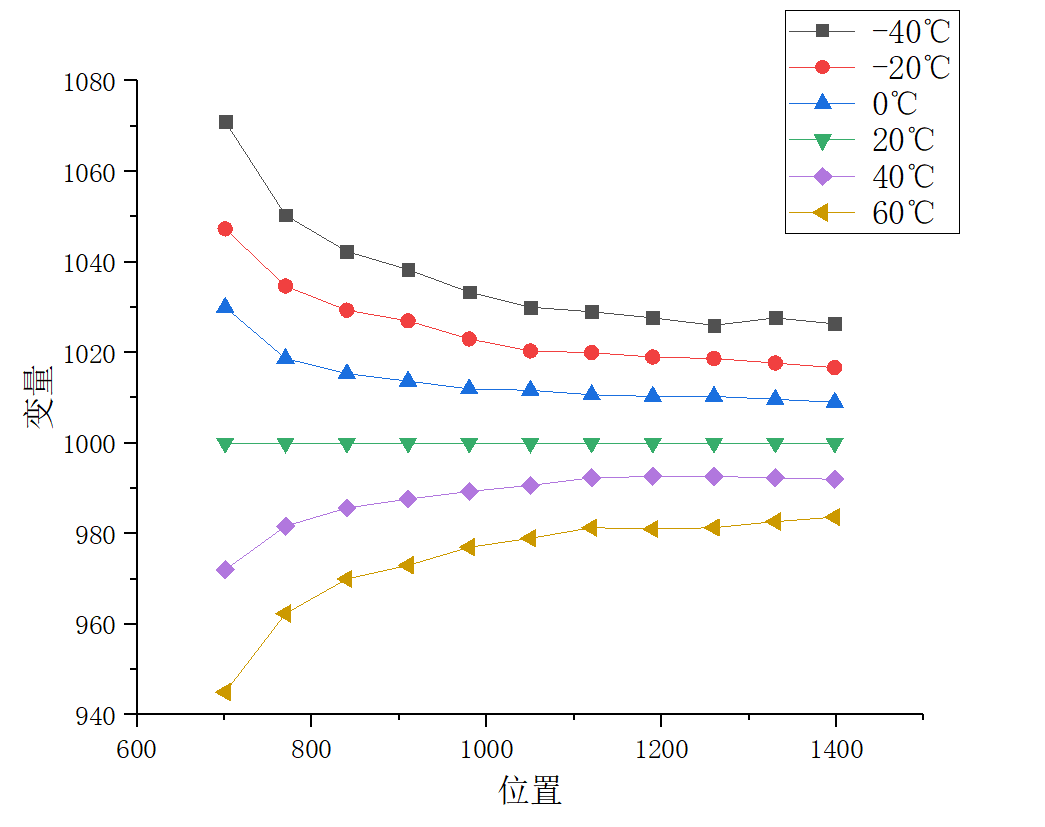
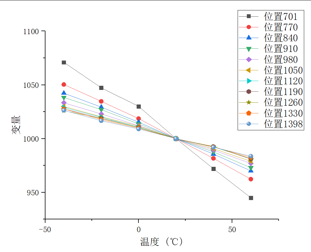
   At this time, it can be seen that the relationship between temperature and variables is linear, while the relationship between position and variables is obviously nonlinear.
2. Use Origin for preliminary fitting. As an excellent data processing software, Origin is very suitable for preliminary fitting of data. Linear fitting is relatively simple and will not be repeated here. When selecting nonlinear fitting, the software will provide preview according to the function we select. The function selected here is
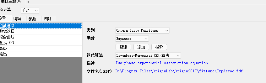
   The fitting effect of this function is very good. Nonlinear fitting is carried out for the position and variable value at the temperature of - 40 - 200 20 40 60, so as to obtain the fitting function in the report. In this way, the value of the variable can be calculated according to the position at a specific temperature
   3. Next, we want to calculate the value of the variable according to the position at each temperature. We know that we do not know the data interval of the temperature, so it is impossible to input specific data in Origin, so we use matlab for calculation. The idea is: according to the linear relationship between temperature and variables, get the temperature at a specific temperature interval (custom temperature interval). Then fit each column of data to get the relationship between position and variables at a certain temperature. At this time, enter the position to get the variables predicted by the software.
   4. Relevant codes are as follows:
   Code snippet 1:

// position.m
%Through data analysis, the relationship between variables and position at a specific temperature can be obtained(Program according to the experimental fitting data)
T_up=input('Upper temperature limit:\n');T_down=input('Lower temperature limit:\n');T_bet=input('Temperature interval:\n');%Input upper and lower temperature limits, temperature interval
L=T_down:T_bet:T_up;T_long=length(L);
Data=zeros(11,T_long);
for i=1:11
    j=630+70*i;
    Data(i,1)=j;
end
for i=1:T_long
    T=T_down+(i-1)*T_bet;
    Data(1,i)=1023.54603-1.26571*T;
    Data(2,i)=1016.76825-0.88238*T;
    Data(3,i)=1014.36825-0.72571*T;
    Data(4,i)=1013.15873-0.65476*T;
    Data(5,i)=1011.41587-0.56381*T;
    Data(6,i)=1010.35873-0.50381*T;
    Data(7,i)=1010.29841-0.47429*T;
    Data(8,i)=1009.72063-0.46095*T;
    Data(9,i)=1009.28571-0.44524*T;
    Data(10,i)=1009.4381-0.44381*T;
    Data(11,i)=1008.84444-0.42333*T;%The above is based on origin Calculate the corresponding variables according to the fitting results
% Q=zeros(1,11);%Create an array of storage locations
% for i=1:11
%     j=630+70*i;
%     Q(1,i)=j;
% end
end
% Data=zeros(1,11);%An array that stores variables
% Data(2,1)=1023.54603-1.26571*T;
% Data(2,2)=1016.76825-0.88238*T;
% Data(2,3)=1014.36825-0.72571*T;
% Data(2,4)=1013.15873-0.65476*T;
% Data(2,5)=1011.41587-0.56381*T;
% Data(2,6)=1010.35873-0.50381*T;
% Data(2,7)=1010.29841-0.47429*T;
% Data(2,8)=1009.72063-0.46095*T;
% Data(2,9)=1009.28571-0.44524*T;
% Data(2,10)=1009.4381-0.44381*T;
% Data(2,11)=1008.84444-0.42333*T;

Code snippet 2
cftool tool is used in nonlinear fitting with matlab. matlab's own fitting tool can automatically generate code, so we can call the generated code directly. It should be noted that matlab will draw after fitting. When fitting thousands of groups of data, drawing thousands of diagrams is obviously unrealistic, so it needs to be modified slightly.

// createFit.m
function [fitresult, gof] = createFit(xdata, ydata)
%CREATEFIT(XDATA,YDATA)
%  Create a fit.
%
%  Data for 'untitled fit 1' fit:
%      X Input : xdata
%      Y Output: ydata
%  Output:
%      fitresult : a fit object representing the fit.
%      gof : structure with goodness-of fit info.
%
%  See also  FIT, CFIT, SFIT.

%  from MATLAB On 18-Aug-2021 16:31:40 Automatic generation


%% Fit: 'untitled fit 1'.
[xData, yData] = prepareCurveData( xdata, ydata );

% Set up fittype and options.
ft = fittype( 'exp2' );
opts = fitoptions( 'Method', 'NonlinearLeastSquares' );
opts.Display = 'Off';
opts.StartPoint = [1401.2829718976 -0.000217159328261083 -951.613694229122 -0.00253631457518578];

% Fit model to data.
[fitresult, gof] = fit( xData, yData, ft, opts );

% Plot fit with data.
% figure( 'Name', 'untitled fit 1' );
% h = plot( fitresult, xData, yData );
% legend( h, 'ydata vs. xdata', 'untitled fit 1', 'Location', 'NorthEast' );
% % Label axes
% xlabel xdata
% ylabel ydata
end

Code snippet 3
Through the above, the data fitting is successful, so the last part is data prediction.

// forcast.m
[m,n]=size(Data);
o=700:1:1400;
DATA=zeros(length(o),n);
xdata=700:70:1400;
for i=1:n
    ydata=Data(:,i);
    ydata=ydata';
    createFit(xdata,ydata);
    xdata=700:1:1400;
    DATA(:,i)=ans(xdata);
    xdata=700:70:1400;
end

So far, the batch fitting prediction of data is completed.