1. Bayesian theorem

Bayesian theorem: P ( H ∣ X ) = P ( X ∣ H ) P ( H ) P ( X ) P(H|X)=\frac{P(X|H)P(H)}{P(X)} P(H∣X)=P(X)P(X∣H)P(H)​

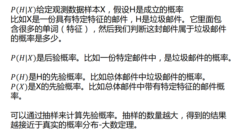
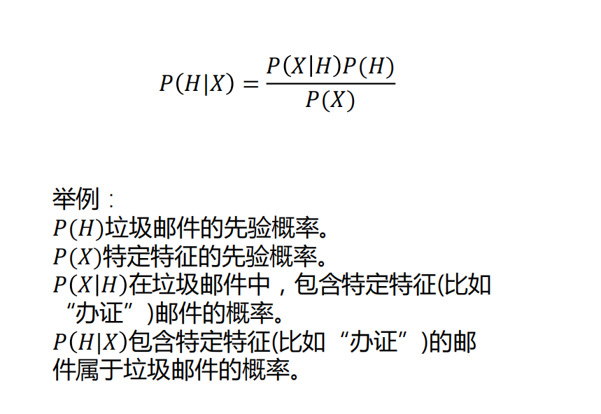
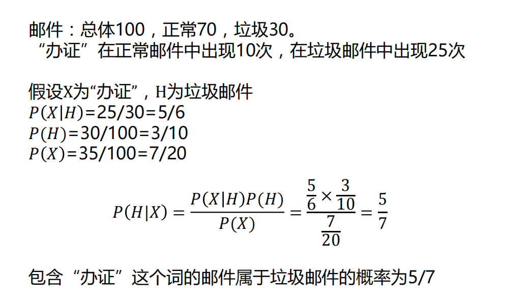
The above is an example of a feature. If there are multiple features, the statistics will be huge, as shown in the following figure. If you need to calculate the impact of certificate processing on spam, you need to calculate the impact of certificate processing + financial pile spam, and the impact of certificate processing + financial management + investment on spam, Calculate the impact of certificate processing + financial management + investment + information on spam... It needs to be calculated in total 2 n − 1 2^{n-1} 2n − 1 time, n is the characteristic number. In this way, if we have many characteristics, it is obviously impossible to complete the calculation.

So we introduce naive Bayes and assume that X1, X2, X3... Are independent of each other
P ( H ∣ X ) = P ( X 1 ∣ H ) P ( X 2 ∣ H ) ... ... P ( X n ∣ H ) P ( H ) P ( X 1 ) P ( X 2 ) ... ... P ( X n ) P(H|X)=\frac{P(X1|H)P(X2|H)......P(Xn|H)P(H)}{P(X1)P(X2)......P(Xn)} P(H∣X)=P(X1)P(X2)......P(Xn)P(X1∣H)P(X2∣H)......P(Xn∣H)P(H)​
However, it is obvious that the characteristics are not independent of each other. In terms of the above four characteristics, investment and financial management are certainly not independent of each other. Investment can be said to be a way of financial management. However, since we assume that the error of the results calculated independently is small, we think that naive Bayes is used for calculation.

2. Centralized Bayesian model

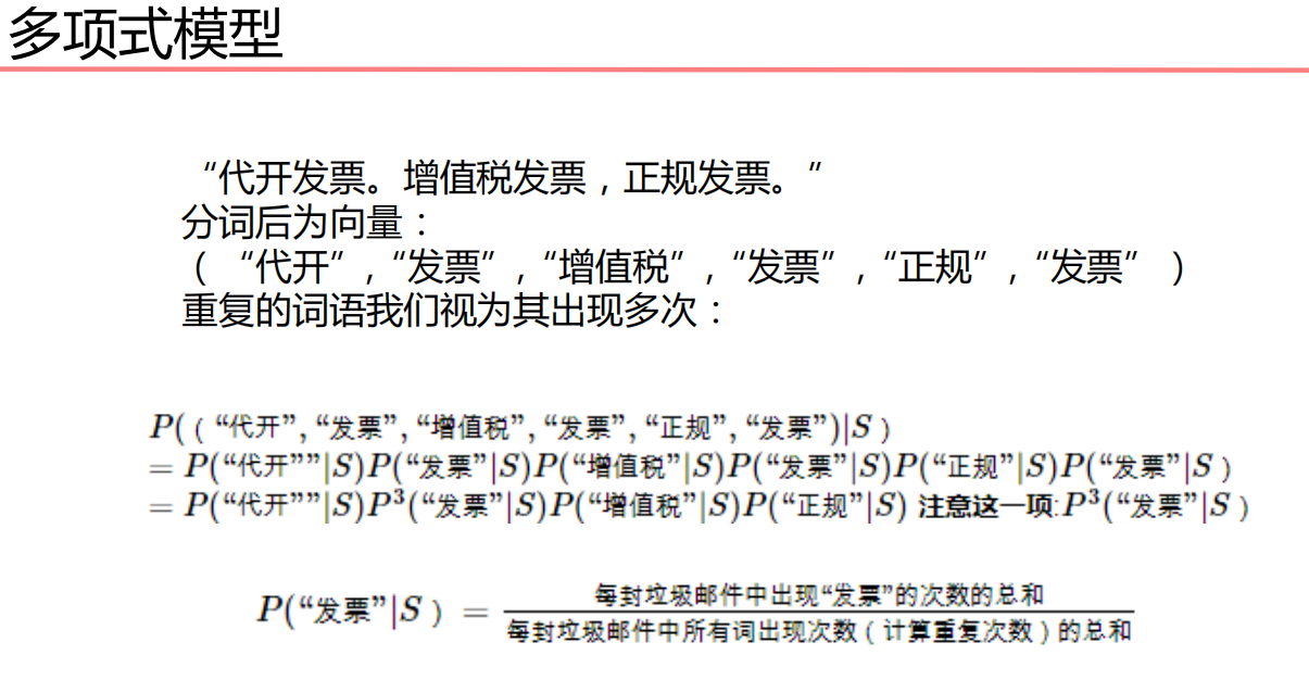
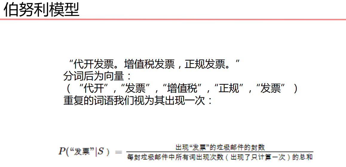
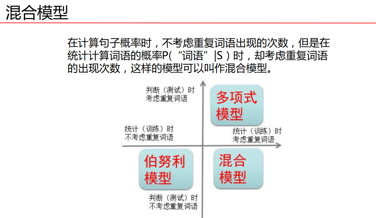
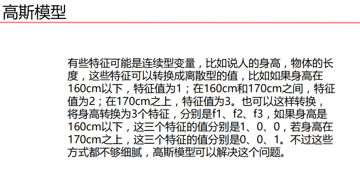
2. Word bag model

Bag of Words model(Bow model) first appeared in the field of natural language processing and information retrieval. The model ignores the elements such as grammar and word order of the text, and regards it only as a collection of several words, and the occurrence of each word in the document is independent. Bow uses a set of unordered words to express a text or a document

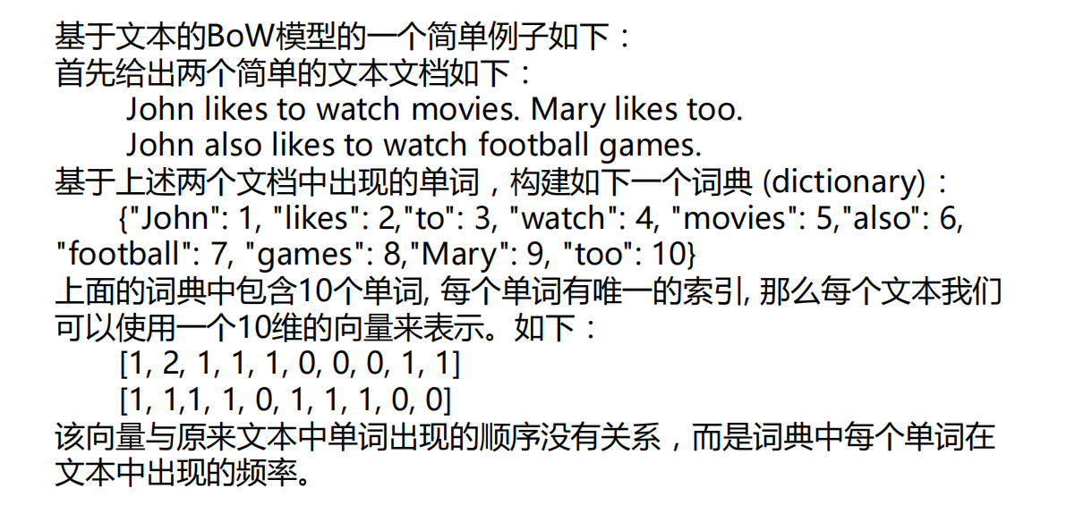
The word bag model is used to convert articles of different lengths into vectors of the same length.

Countvector method is used to construct a word dictionary. Each word instance is converted into a numerical feature of a feature vector. Each element is the number of times a specific word appears in the text

from sklearn.feature_extraction.text import CountVectorizer

texts=['dog cat finsih','dog fish dog','bird','monkey,dog']
model=CountVectorizer()
model_fit=model.fit_transform(texts)

print(model_fit)
print(model.get_feature_names_out())
print(model_fit.toarray())
print(model_fit.toarray().sum(axis=0))#Column direction addition

  (0, 2)	1
  (0, 1)	1
  (0, 3)	1
  (1, 2)	2
  (1, 4)	1
  (2, 0)	1
  (3, 2)	1
  (3, 5)	1
['bird' 'cat' 'dog' 'finsih' 'fish' 'monkey']
[[0 1 1 1 0 0]
 [0 0 2 0 1 0]
 [1 0 0 0 0 0]
 [0 0 1 0 0 1]]
[1 1 4 1 1 1]

3.TF-IDF

Extract article keywords:
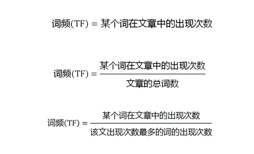
1. Extract Term Frequency (abbreviation TF) The most common words in an article may be "yes, yes, in" and other stop words that are not helpful for article classification or search
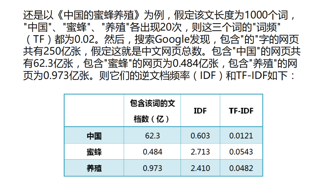
2. Suppose we filter out all the stop words and only consider the meaningful words. You may encounter such a problem. The TF of the three words "China", "bee" and "breeding" are the same. As keywords, are they of the same importance?
3. Obviously not. "China" is a very common word. Relatively speaking, "bee" and "breeding" are not so common. If these three words appear as many times in an article, it is reasonable to think that "bee" and "breeding" are more important than "China", and "breeding" and "bee" should rank first in China in terms of keyword ranking.
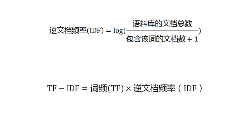
So we need an importance adjustment coefficient to measure whether a word is a common word. If a word is rare, but it appears many times in this article, it is likely to reflect the characteristics of this article, which is the keyword we need.

Expressed in statistical language, it is necessary to assign a "importance" weight to each word on the basis of word frequency. The most common word "in" is given the smallest weight, and the more common word "China" is given a smaller weight. The less common words "bee" and "breeding" give greater weight. This weight is called "inverse document frequency", abbreviated as IDF. Its size is inversely proportional to the frequency of a word.
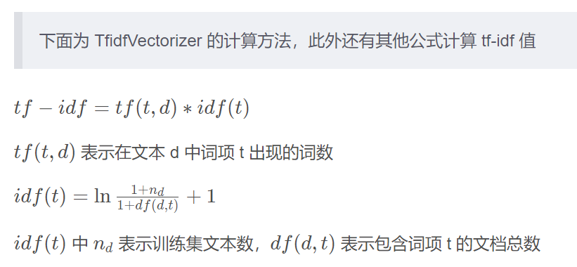
Method of calculating word frequency:

from sklearn.feature_extraction.text import TfidfVectorizer

text=['dog bird','dog cat','the ','fox']
model_tif=TfidfVectorizer(norm=None)#If norm is set to none, the calculation result will be the same as the picture above
model_tif.fit(text)

print(model_tif.vocabulary_)
print(model_tif.idf_)#Calculate the IDF vector, and the position sequence number of each element corresponds to the dictionary value
vector=model_tif.fit_transform(text)#Calculate RF-IDF
print(vector.toarray())

{'dog': 2, 'bird': 0, 'cat': 1, 'the': 4, 'fox': 3}
[1.91629073 1.91629073 1.51082562 1.91629073 1.91629073]
[[1.91629073 0.         1.51082562 0.         0.        ]
 [0.         1.91629073 1.51082562 0.         0.        ]
 [0.         0.         0.         0.         1.91629073]
 [0.         0.         0.         1.91629073 0.        ]]