1, Bayesian decision theory

1. Probability and statistics

(1) Probability: know a model and corresponding parameters, and predict the results and characteristics (such as mean, variance, covariance, etc.) produced by the model, i.e. data;
(2) Statistics: predict the model and corresponding parameters according to the existing data;
It can be seen that the purpose of probability and statistics is the opposite;

2. Probability function and likelihood function

For functions P ( x ∣ θ ) P\left( x|\theta \right) P(x∣ θ)， There are two inputs, x x x represents a specific data, θ \theta θ Represent model parameters; Then there are two situations:
(1) x x x change, θ \theta θ When the model and parameters are fixed, different samples are given x x x. So what you get is x x What is the probability of x? This is the probability function;
(2) x x x fixed, θ \theta θ In the case of change, it is calculated for different model parameters θ \theta θ， What is the probability of x this sample point? This is the likelihood function (possibility).

3. Bayesian formula

P ( A ∣ B ) = P ( A ) P ( B ∣ A ) P ( B ) P\left( A|B \right) =\frac{P\left( A \right)P\left( B|A \right) }{P\left( B \right)} P(A∣B)=P(B)P(A)P(B∣A)​
There is A causal relationship between events in Bayesian formula. If A is the cause and B is the result, that is, A is one of the causes of B; Then:

1. P ( A ∣ B ) P\left( A|B \right) P(A ∣ B) is called A posteriori probability, which is A consequence probability, that is, after event B has occurred, how likely it is that A causes B to occur, which can be understood as how sure you can believe A piece of evidence (or how sure you can determine that A causes B to occur);
2. P ( A ) P(A) P(A) is called a priori probability, that is, the probability that can be obtained directly from previous experience and analysis. For example, if we throw a normal coin, we can know that the probability of facing up is 0.5 a priori according to experience;
3. P ( B ∣ A ) P\left( B|A \right) P(B ∣ A) is called class conditional probability, which can be understood as if A A A happens, then next B B B how likely is it to occur, e.g A A A = 'today is May Day', B B B = 'today's Holiday', then P ( B ∣ A ) = 1 P(B|A)=1 P(B∣A)=1； Or likelihood.
4. P ( B ) P(B) P(B) is the "evidence" factor used for normalization, i.e. leading to B B B is a collection of all possibilities that occur, such as B B B = 'today's Holiday', then P ( B ) P(B) P(B) is a collection of all the possibilities that may lead to today's holiday, such as today's weekend or may day, for an event B B B. Usually P(B) is a definite value.
   Explanation of full probability formula and Bayesian formula in probability theory and mathematical statistics:
   
5. Understanding Bayesian formula from two perspectives
   (1) The Bayesian formula can be reduced to:
   P ( A ∣ B ) = P ( A ) P ( B ∣ A ) P ( B ∣ A ) P ( A ) + P ( B ∣ ∼ A ) P ( ∼ A ) P\left( A|B \right) =\frac{P\left( A \right) P\left( B|A \right)}{P\left( B|A \right) P\left( A \right) +P\left( B|\sim A \right) P\left( \sim A \right)} P(A∣B)=P(B∣A)P(A)+P(B∣∼A)P(∼A)P(A)P(B∣A)​
   If we want to say that the proposition "today is a holiday, then today is May Day" is true, we can think of what to do, as long as we make the denominator of the above Bayesian formula P ( B ∣ ∼ A ) P ( ∼ A ) P\left( B|\sim A \right) P\left( \sim A \right) P(B ∣∼ A)P(∼ A) is 0, that is, other possible factors other than may day that cause the holiday are excluded; But obviously, this proposition is false, because there are more than one factor causing the holiday;
   So we can conclude that all factors should be considered when making judgment. If today is a holiday, but today is not necessarily may day, it is more likely to be a weekend;
   (2) From P ( A ) P(A) From the perspective of P(A): we assume A A A and B B B closely related, take the extreme case order P ( B ∣ A ) = 1 P(B|A)=1 P(B ∣ A)=1, i.e. if A A A happens, then B B B must occur; But even in this case, if P ( A ) P(A) P(A) is too small, so combined P ( A ∣ B ) P(A|B) P(A ∣ B) will also be small; For example, for those millions of lottery tickets, once someone wins, he must have become a millionaire at that time; But in fact, only very few of all millionaires have won the million lottery; So we can know that even if a factor is strongly related to the result, when the probability of this factor is very low, we should carefully consider whether it is caused by other factors.

4. Bayesian decision theory

Bayesian decision theory is a basic method to implement decision under the framework of probability. It considers selecting the optimal category marker based on the known correlation probability and misjudgment loss.
Suppose there are N possible category markers, i.e y = { c 1 , c 2 , . . . , c N } y=\left\{ c_1,c_2,...,c_N \right\} y={c1​,c2​,...,cN​}， λ i j \lambda _{ij} λ ij # is to mark a real as c j {c_j} Sample of cj + x x x misclassified as c i c_i ci ， expected loss (conditional risk)
R ( c i ∣ x ) = ∑ j = 1 N λ i j P ( c j ∣ x ) R\left( c_i|x \right) =\sum_{j=1}^N{\lambda _{ij}P\left( c_j|x \right)} R(ci​∣x)=j=1∑N​λij​P(cj​∣x)
Our aim is to minimize conditional risk when
λ i j = { 0 , i f    i    =    j 1 , o t h e r w i s e \lambda _{ij}=\begin{cases} 0, if\,\,i\,\,=\,\,j\\ 1, otherwise\\ \end{cases} λij​={0,ifi=j1,otherwise​
Conditional risk at this time R ( c ∣ x ) = 1 − P ( c ∣ x ) R\left( c|x \right) =1-P\left( c|x \right) R(c ∣ x)=1 − P(c ∣ x), the Bayesian optimal classifier to minimize the classification error rate is h ∗ ( x ) = a r g max ⁡ c ∈ y P ( c ∣ x ) h^*\left( x \right) =\underset{c\in y}{arg\max}P\left( c|x \right) h∗(x)=c∈yargmax​P(c∣x)
That is, for each sample x x x. Select a posteriori probability P ( c ∣ x ) P(c|x) P(c ∣ x) is the largest category mark. The methods include maximum likelihood estimation and maximum a posteriori probability estimation.
(this part comes from watermelon book)

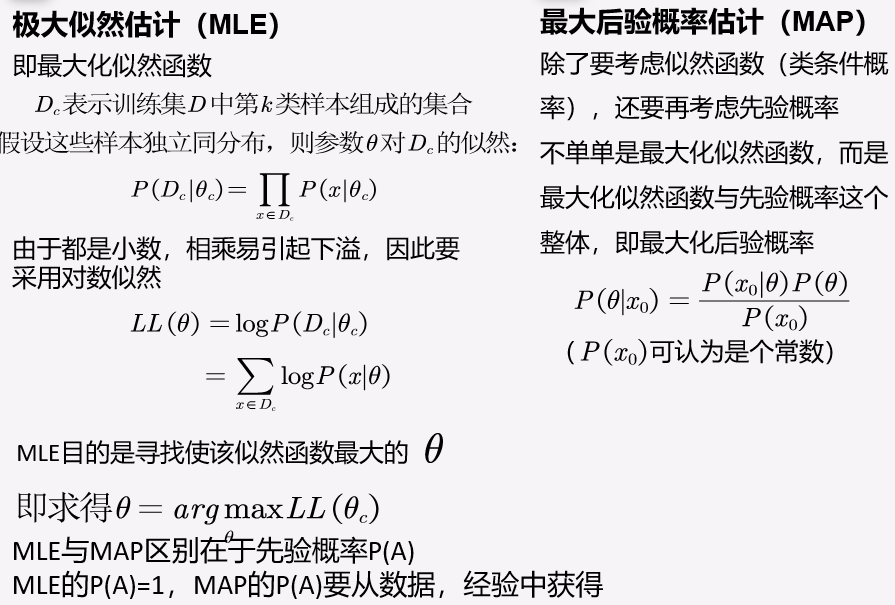
5. Maximum likelihood estimation (MLE) and maximum a posteriori probability estimation (MAP)

2, Naive Bayesian classifier

1. Introduction

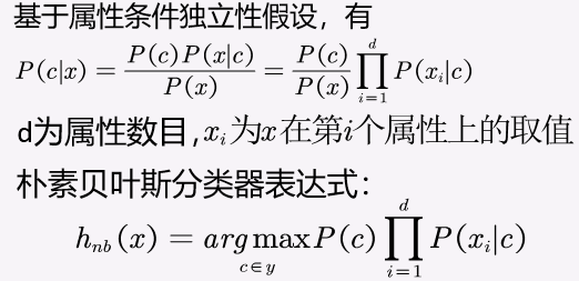
For a posteriori probability P(c|x), the class conditional probability P(x|c) is the joint probability on all attributes, and there is influence between attributes; In order to simplify the problem, naive Bayesian classifier assumes that all attributes are independent of each other, that is, each attribute has an independent impact on the classification results

2. Algorithm representation

3. Code implementation

The training of discrete attributes and continuous attributes should be treated differently

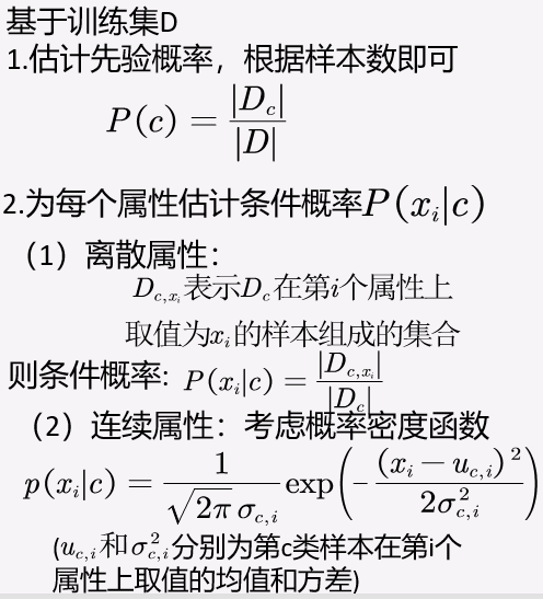
Continuous attributes:

import numpy as np#Iris, three categories, each with 50 samples
import random
import math
def data_split(data):#The original data is divided into a training set with 120 samples and a test set with 30 samples
    data = data[1:]
    train_ratio = 0.8
    train_size = int(len(data) * train_ratio)
    random.shuffle(data)
    train_set = data[:train_size]
    test_set = data[train_size:]
    return train_set, test_set

def class_separate(data_set):#Process, classify and count the data
    separated_data = {}
    data_info = {}#It indicates the corresponding quantity of each kind of flower
    for data in data_set:
        if data[-1] not in separated_data:#Create a new dictionary index. The data and info dictionaries have three indexes respectively, that is, the variety of flowers
            separated_data[data[-1]] = []
            data_info[data[-1]] = 0
        separated_data[data[-1]].append(data)#Divide all flowers into three categories, and each flower will be added to the corresponding flower category
        data_info[data[-1]] += 1
    if 'Species' in separated_data:
        del separated_data['Species']
    if 'Species' in data_info:
        del data_info['Species']
    return separated_data, data_info

def prior_prob(data, data_info):#Calculate the a priori probability of each class
    data_prior_prob = {}
    data_sum = len(data)
    for cla, num in data_info.items():
        data_prior_prob[cla] = num / float(data_sum)
    return data_prior_prob

def mean(data):#Find the mean
    data = [float(x) for x in data]#String to number
    return sum(data) / len(data)

def var(data):#Find variance
    data = [float(x) for x in data]
    mean_data = mean(data)
    var = sum([math.pow((x - mean_data), 2) for x in data]) / float(len(data) - 1)
    return var

def prob_dense(x, mean, var):#Since the sample attribute is a continuous value, the probability density is used
    exponent = math.exp(math.pow((float(x) - mean), 2) / (-2 * var))
    p = (1 / math.sqrt(2 * math.pi * var)) * exponent
    return p

def attribute_info(data):#The mean and variance of the four attributes are calculated respectively
    dataset = np.delete(data, -1, axis = 1) #delete a tap
    result = [(mean(att), var(att)) for att in zip(*dataset)]#zip decomposes the meta group and generates the results of four attributes
    return result

def summarize_class(data):
  data_separated, data_info = class_separate(data)
  summarizeClass = {}
  for index, x in data_separated.items():#The three categories correspond to 4 attributes, a total of 12 groups, and each group contains the corresponding mean and variance
      summarizeClass[index] = attribute_info(x)
  return summarizeClass

def cla_prob(test, summarizeClass):#At this time, summarizeClass is the probability density function parameters of the three categories, i.e. model parameters, and test is the test data (sample data)
  prob = {}
  for cla, summary in summarizeClass.items():#cla category. summary is the set of four attributes (mean and variance) corresponding to this category
      prob[cla] = 1
      for i in range(len(summary)):#Number of attributes
          mean, var = summary[i]
          x = test[i]
          p = prob_dense(x, mean, var)#Calculate the conditional probability of discrete attribute values
      prob[cla] *= p #Finally, we get the conditional probability of this class about all attributes
  return prob#Obtain conditional probability

def bayesian(input_data, data, data_info):#We only need to consider the numerator of Bayesian formula, because the denominator is the same, that is, we only need to consider a priori probability and conditional probability
  priorProb = prior_prob(data, data_info)
  data_summary = summarize_class(data)
  classProb = cla_prob(input_data, data_summary)
  result = {}
  for cla, prob in classProb.items():
      # print(type(classProb))
      p = prob * priorProb[cla]
      result[cla] = p
  return max(result, key=result.get)

iris = np.array(np.loadtxt("IrisData.csv", dtype=str, delimiter=",")).tolist()##There are 150 samples for importing iris data, including four attributes and three categories (0,1,2), and each category has 50 samples
train_set, test_set = data_split(iris)
train_separated, train_info = class_separate(train_set)#Obtain the classified data and the number of samples in each category
correct = 0
for x in test_set:
  input_data = x[:-1]
  label = x[-1]
  result = bayesian(input_data, train_set, train_info)
  if result == label:
      correct += 1
print("precision: ", correct / len(test_set))

Training results: