1. Problems of genetic algorithm
1. In the process of selection, how many times will it reduce the population? What if it is repeated?
There is no limit to the number of choices, that is, there will be no choices. Therefore, the population will be reduced, and the repeated individuals will be abandoned and re selected. It is suggested that the number of choices should be less than the number of populations, because there is no repetition. Therefore, when the number of choices is the number of populations, all choices will be made, which will lose the significance of selection. The reason for abandoning repetition is that repeated individuals do not help the differentiation of the population (imagine that in extreme cases, all repeated individuals are the same after crossing, which is meaningless).
2. Once the fitness of each individual in the population is calculated, why not directly select the one with high fitness, abandon the one with low fitness, and use other algorithms?
Individuals with low fitness may also have high-quality genes. Real life example: a pair of fools gave birth to a clever son.
3. Is the crossing process random or pairwise? How many times is it appropriate?
Random or pairwise crossover is allowed, and the number of crossover is greater than or equal to the number of individuals in the initial population / 2. Because the crossover produces two new individuals at a time, and the variation in step 3 does not produce new individuals, in order to ensure that the number of individuals in the population will not be less and less (negative population growth), the number of crossover is greater than or equal to the number of individuals in the initial population / 2.
Genetic algorithm implemented in JAVA: http://www.theprojectspot.com/tutorial-post/creating-a-genetic-algorithm-for-beginners/3
Using GA to solve TSP problem: http://www.theprojectspot.com/tutorial-post/applying-a-genetic-algorithm-to-the-travelling-salesman-problem/5
Genetic algorithm tutorial: http://www.w3ii.com/genetic_algorithms/default.html
2. Scikit opt - SA (simulated annealing)
1.Simulated annealing algorithm can be divided into three parts: solution space, objective function and initial solution.

2.Basic idea of simulated annealing:
	(1) Initialization: initial temperature T(Fully large),Initial solution state S(It is the starting point of algorithm iteration),each T Number of iterations of value L
	(2) yes k=1, ..., L Do the first(3)Go to step 6:
	(3) Generate new solutions S′
	(4) Calculation incrementΔT=C(S′)-C(S),among C(S)Cost function
	(5) ifΔT<0 Then accept S′As a new current solution, otherwise in probability exp(-ΔT/T)accept S′As a new current solution.
	(6) If the termination conditions are met, the current solution is output as the optimal solution and the program is ended.
	The termination condition is usually taken as terminating the algorithm when several new solutions in succession are not accepted.
	(7) T Gradually reduced, and T->0,Then turn to step 2.
2.1SA finding the maximum value of function
2.1.1 definition questions
demo_func = lambda x: x[0] ** 2 + (x[1] - 0.05) ** 2 + x[2] ** 2
2.1.2 execute SA
from sko.SA import SA

sa = SA(func=demo_func, x0=[1, 1, 1], T_max=1, T_min=1e-9, L=300, max_stay_counter=150)
best_x, best_y = sa.run()
print('best_x:', best_x, 'best_y', best_y)
# best_x: [-2.09849560e-05  5.00075424e-02  2.40334265e-06] best_y 5.030317095901513e-10
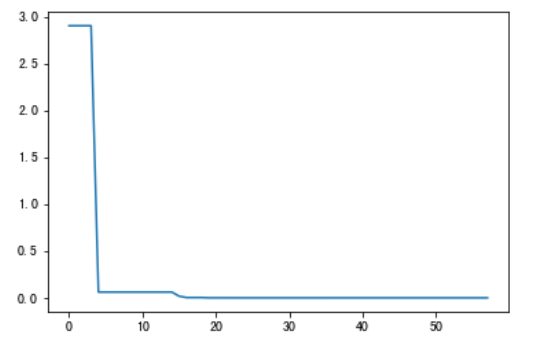
2.1.3 drawing results
import matplotlib.pyplot as plt
import pandas as pd

plt.plot(pd.DataFrame(sa.best_y_history).cummin(axis=0))
plt.show()
Moreover, scikit opt provides three types of simulated annealing: fast, Boltzmann and Cauchy. See more SA
2.2SA solving TSP problems
2.2.1 definition questions
import sys
import numpy as np
from scipy import spatial
import matplotlib.pyplot as plt


file_name = 'nctu.txt'
points_coordinate = np.loadtxt(file_name, delimiter=',')
num_points = points_coordinate.shape[0]
distance_matrix = spatial.distance.cdist(points_coordinate, points_coordinate, metric='euclidean')
distance_matrix = distance_matrix * 111000  # 1 degree of lat/lon ~ = 111000m


def cal_total_distance(routine):
    '''The objective function. input routine, return total distance.
    cal_total_distance(np.arange(num_points))
    '''
    num_points, = routine.shape
    return sum([distance_matrix[routine[i % num_points], routine[(i + 1) % num_points]] for i in range(num_points)])
2.2.2 SA for TSP
from sko.SA import SA_TSP

sa_tsp = SA_TSP(func=cal_total_distance, x0=range(num_points), T_max=100, T_min=1, L=10 * num_points)

best_points, best_distance = sa_tsp.run()
print(best_points, best_distance, cal_total_distance(best_points))
2.2.3 drawing results
# %% Plot the best routine
from matplotlib.ticker import FormatStrFormatter

fig, ax = plt.subplots(1, 2)

best_points_ = np.concatenate([best_points, [best_points[0]]])
best_points_coordinate = points_coordinate[best_points_, :]
ax[0].plot(sa_tsp.best_y_history)
ax[0].set_xlabel("Iteration")
ax[0].set_ylabel("Distance")
ax[1].plot(best_points_coordinate[:, 0], best_points_coordinate[:, 1],
           marker='o', markerfacecolor='b', color='c', linestyle='-')
ax[1].xaxis.set_major_formatter(FormatStrFormatter('%.3f'))
ax[1].yaxis.set_major_formatter(FormatStrFormatter('%.3f'))
ax[1].set_xlabel("Longitude")
ax[1].set_ylabel("Latitude")
plt.show()

2.2.4 drawing animation
# %% Plot the animation
import matplotlib.pyplot as plt
from matplotlib.animation import FuncAnimation
from matplotlib.ticker import FormatStrFormatter

best_x_history = sa_tsp.best_x_history

fig2, ax2 = plt.subplots(1, 1)
ax2.set_title('title', loc='center')
line = ax2.plot(points_coordinate[:, 0], points_coordinate[:, 1],
                marker='o', markerfacecolor='b', color='c', linestyle='-')
ax2.xaxis.set_major_formatter(FormatStrFormatter('%.3f'))
ax2.yaxis.set_major_formatter(FormatStrFormatter('%.3f'))
ax2.set_xlabel("Longitude")
ax2.set_ylabel("Latitude")
plt.ion()
p = plt.show()


def update_scatter(frame):
    ax2.set_title('iter = ' + str(frame))
    points = best_x_history[frame]
    points = np.concatenate([points, [points[0]]])
    point_coordinate = points_coordinate[points, :]
    plt.setp(line, 'xdata', point_coordinate[:, 0], 'ydata', point_coordinate[:, 1])
    return line


ani = FuncAnimation(fig2, update_scatter, blit=True, interval=25, frames=len(best_x_history))
plt.show()

ani.save('sa_tsp.gif', writer='pillow')
2.3 complete code and data
Download link: https://pan.baidu.com/s/18OySLiJx3E9_53TA2PO3Sw Extraction code: 06gq