Section 1 Introduction to spark

1. What is spark?

1.apache spark is a unified computing engine and a set of class libraries. Using spark to process data is 100 times faster than the traditional way.
2. It is not that spark is 100 times faster than python on a single computer, but that spark is mainly used for parallel data processing on computer clusters (clusters are not three or five machines for programs, but a large machine, which is implemented by cluster software).
3.spark is currently the most active open source engine and the standard tool for any developer or data scientist interested in big data.

2. spark architecture diagram

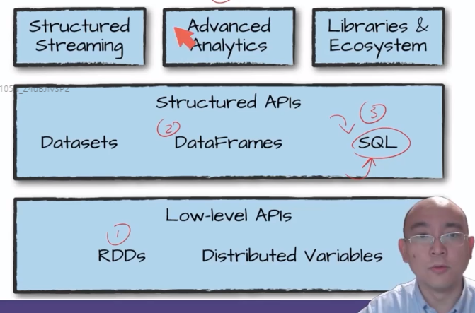
The dataframe of spark is the same as that of python, but the dataframe here can span multiple machines.

3. Installation and download of spark

Note before installation: make sure java is installed on the computer and python 3.7 uses spark 2.4 in this lesson 5.
Installation package: wechat installation package can be added.

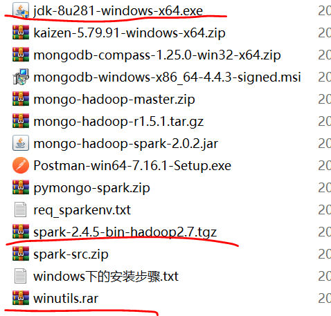
The installation steps are as follows:

1. Install jdk

2. Set environment variable - JAVA_HOME variable

JAVA_HOME= D:\SoftInStall\java\jdk1.8

3. Install winutils settings - HADOOP_HOME variable settings
HADOOP_HOME =D:\SoftInStall\winutils

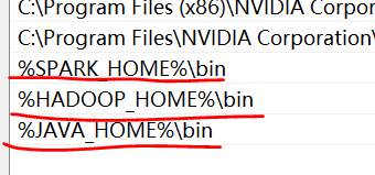
4. Decompress the spark package and set SPARK_HOME variable
SPARK_HOME=D:\SoftInStall\spark-2.4.5

5. Activate all three settings in the path variable of the system.

6. It is important to adjust the system python 3.8 to 3.7.
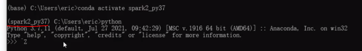
(1) Open python to determine the version.
(2) cmd run under the root directory

1. To create a virtual environment:
   conda create -n sparkenv2 python=3.7
   -n is the meaning of the name, that is, sparkenv2 is a name.
2. Activate environment:
   conda activate sparkenv2
   Close the environment conda deactivate
   
   conda env list can view the current number of environments.
3. The following software is installed in sparkenv2, a virtual environment:
   pip install jupyter numpy pandas matplotlib findspark

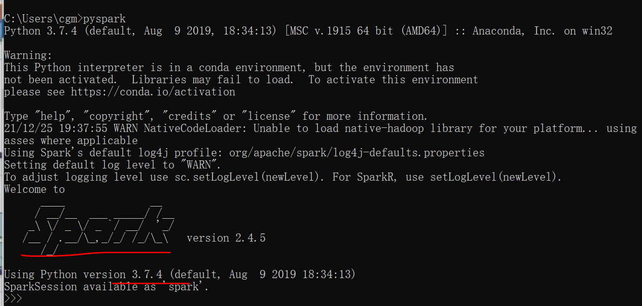
7. Enter spark virtual environment.
pyspark

ctrl+z to exit the environment.

Section 2 RDD of spark (elastic distributed data)

1.RDD (resilient distributed dataset) refers to a read-only and partitioned distributed dataset. All or part of this dataset can be cached in memory and reused between multiple calculations.
resilient can be revived. After one machine hangs up, data can be revived on other machines.
2. It is a special set with fault-tolerant mechanism, which can be distributed on cluster nodes to carry out various parallel operations in the way of functional programming operation set.

1. RDD creation

#Environment required for configuring spark
import findspark
findspark.init()
#Activate the native spark environment
import pyspark
#Import the environment required by spark (SparkConf and SparkContext), and then load the data.
from pyspark import SparkConf,SparkContext
sc=SparkContext(conf=SparkConf().setAppName("gm").setMaster("local"))

lines=sc.textFile("word_count.text",3)  #lines is an rdd
#take in spark is similar to head in df
lines.take(1)

2. flatMap is used to count the frequency of words

Use the function of spark to count the number of words in this file and the frequency of words
#Line by line processing has three main functions in spark
Use the map function one by one
filter function with less than one row
One line multi line output flatmap function

1.map one in and one out
2.flatMap processes each row of data, and the output result can be one row or multiple rows.
3.filter filtering

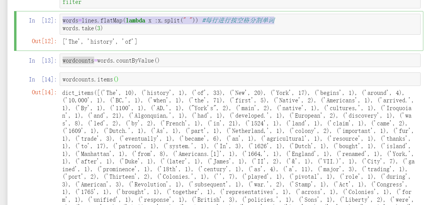
words=lines.flatMap(lambda x :x.split(" ")) #Separate words by spaces on each line
wordcounts=words.countByValue()
wordcounts.items()

What can flatMap do? The original python is a processor processing line by line, and other processors rest. Now it is divided into three parts. It takes three processors to work at the same time. What the three processors do mainly depends on the contents in the brackets of flatMap. (for example, the canteen used to have one window, but now there are 10 windows. spark is such a distributed framework)

3. Dataset consolidation (filter and map)

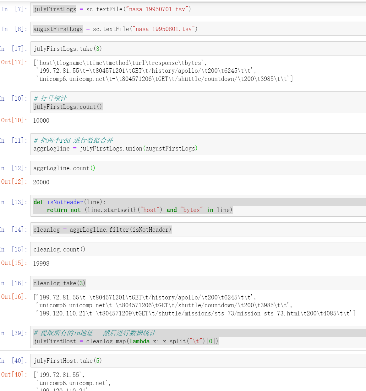
julyFirstLogs = sc.textFile("nasa_19950701.tsv")
augustFirstLogs = sc.textFile("nasa_19950801.tsv")
julyFirstLogs.count() #Output 10000
# Merge the two RDDS
aggrLogline = julyFirstLogs.union(augustFirstLogs)
# 1. Delete the first line
def isNotHeader(line):
    return not (line.startswith("host") and "bytes" in line)
 cleanlog = aggrLogline.filter(isNotHeader)

# 2. Extract all ip addresses and then make data statistics 
julyFirstHost = cleanlog.map(lambda x: x.split("\t")[0])
julyFirstHost.take(5)
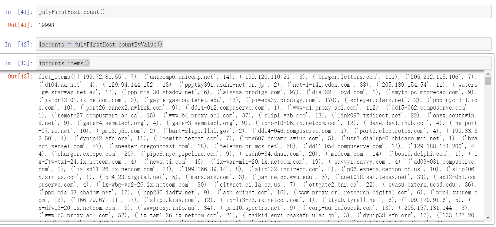
# 3. Statistics
ipcounts = julyFirstHost.countByValue()
ipcounts.items()
# 4. Data saving
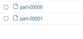
julyFirstHost.saveAsTextFile('out/hosts')

#Saved files (spark has two CPUs by default):

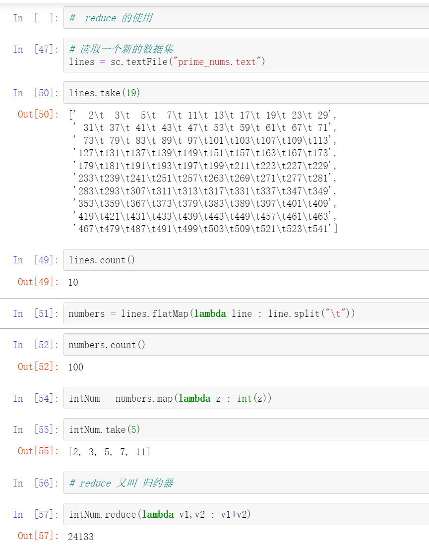
4. reduce - reducer

Let each machine add first, and then each machine add again. The data can be distributed on different machines.

Section 3 dataframe operation of spark

spark's dataframe is a distributed data collection and a high-level API. Compared with the underlying API, RDD has more functions and data security.

# Start spark environment
import findspark
findspark.init()
from pyspark.sql import SparkSession
spark=SparkSession.builder.appName('Dataframe').getOrCreate()

1.Schema mode

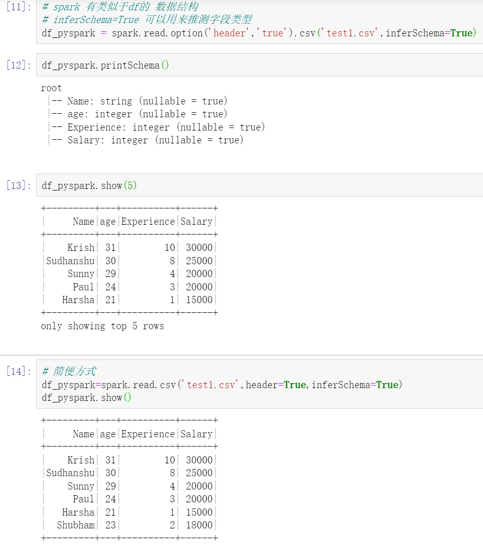
# spark has a data structure similar to df
# Inforschema = true can be used to infer field types
df_pyspark = spark.read.option('header','true').csv('test1.csv',inferSchema=True)
df_pyspark.printSchema() #Look at the field
df_pyspark.show(5)   #The head of show and pandas are unreadable

# Simple way
df_pyspark=spark.read.csv('test1.csv',header=True,inferSchema=True)
df_pyspark.show() 

2. Filter different columns

df_pyspark.select(['Name']).show(5)

3.describe

df_pyspark.describe().show()

4. Add field

df_pyspark = df_pyspark.withColumn('new',df_pyspark['Experience']+5)

5. Delete column

#A value must be assigned, or deletion will be invalid
df_pyspark=df_pyspark.drop('new')

6. Rename data

# Rename data * * * Note
# The save and show functions cannot be used at the same time. Either show is used for real-time display, or assign a value, and then show is used for the next line
df_pyspark2=df_pyspark.withColumnRenamed('Name','New Name')
df_pyspark2.show()

7. Delete null value

In pandas, we use fillna and dropna to process null data, so how to delete the null part in the column?

1. df_pyspark.na.drop().show()
2. The hidden mode uses how to distinguish how to delete null values. how == any
   df_pyspark.na.drop(how="any").show()
3. How many valid values can there be in a row with thresh=1
   df_pyspark.na.drop(how="any",thresh=1).show()
   4. When we delete the na value, can the null value be on a column
   df_pyspark.na.drop(how=“any”,subset=[‘Age’,‘Salary’]). show() if age and salary are null, they will be deleted.

8. Fill in null values

1.df_pyspark.na.fill(0,['Experience','age']).show()
2. The above are single column or global processing. If data customization is required, the following functions are adopted to introduce the module imputer

from pyspark.ml.feature import Imputer
imputer = Imputer(
    inputCols=['age', 'Experience', 'Salary'], 
    outputCols=["{}_imputed".format(c) for c in ['age', 'Experience', 'Salary']]
    ).setStrategy("median")
imputer.fit(df_pyspark).transform(df_pyspark).show()

9. For data type conversion, you can use withcolum method to call cast function

df_pyspark = df_pyspark.withColumn("age",df_pyspark.age.cast('double'))

10. Conditional filtering

1. Line filtering

1.df_pyspark.filter("Salary<=20000").show()
2.df_pyspark.filter(df_pyspark['Salary']<=20000).show()

2. Row filtering plus column filtering

df_pyspark.filter("Salary<=20000").select(['Name','age']).show()

3. Multi condition screening

# Multiple conditions. Each condition must be enclosed in parentheses and linked with and or  
# and yes & or yes in spark|
df_pyspark.filter((df_pyspark['Salary']<=20000) & (df_pyspark['Salary']>15000) ).show()

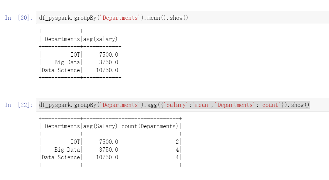
11. Data summary

For data aggregation using the group by function, aggregation functions must be provided, such as summation and average
1.df_pyspark.groupBy('Departments').sum().show()
2.df_pyspark.groupBy('Name').sum().show()
3.df_pyspark.groupBy('Name').avg().show()
4.df_pyspark.groupBy('Departments').mean().show()
5. Multiple statistical functions:

df_pyspark.groupBy('Departments').agg({'Salary':'mean','Departments':'count'}).show()

Section 4 Spark SQL operation

df is convenient for machine learning. SQL is not convenient for machine learning, but each has its own necessity.

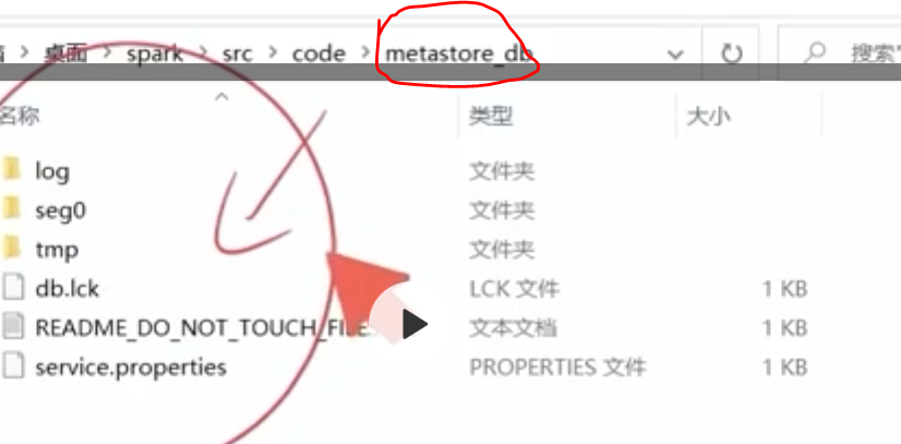
. enableHiveSupport() allows the data table to be saved in the metastore_db folder. Not a one-time temporary table

import findspark
findspark.init()
from pyspark.sql import SparkSession
# . enableHiveSupport() allows the data table to be saved instead of a one-time temporary table
spark = SparkSession.builder.appName('spark-sql').enableHiveSupport().getOrCreate()

df_pyspark=spark.read.json("2015-summary.json")
#Create temporary table
spark.read.json("2015-summary.json").createOrReplaceTempView("some_sql_view")
#Query statement
spark.sql("select * from some_sql_view").show()
spark.sql("select DEST_COUNTRY_NAME,ORIGIN_COUNTRY_NAME from some_sql_view").show(3)
#Table view statement
spark.sql("""
SHOW TABLES""").show()
#Previous statement DEST_COUNTRY_NAME column name
df_pyspark.filter(df_pyspark.DEST_COUNTRY_NAME.like ('S%')).show()
#Current query statement
spark.sql("select DEST_COUNTRY_NAME,ORIGIN_COUNTRY_NAME from some_sql_view where DEST_COUNTRY_NAME like 'S%' ").show(3)

# Group by we need to summarize the data of the destination_ COUNTRY_ Name then calculates the sum 
spark.sql("""
SELECT DEST_COUNTRY_NAME, sum(count)
FROM some_sql_view GROUP BY DEST_COUNTRY_NAME order by sum(count) desc
""").show()

#Create table  # The data just now are temporary data. If we need to use this information for a long time, we can create a table instead of a temporary table
1.spark.sql("""CREATE TABLE flights_csv (
  DEST_COUNTRY_NAME STRING,
  ORIGIN_COUNTRY_NAME STRING COMMENT "remember, the US will be most prevalent",
  count LONG)
USING csv OPTIONS (header true, path '2015-summary.csv')""")
2.spark.sql("""CREATE TABLE flights (
  DEST_COUNTRY_NAME STRING, ORIGIN_COUNTRY_NAME STRING, count LONG)
USING JSON OPTIONS (path '2015-summary.json')""")

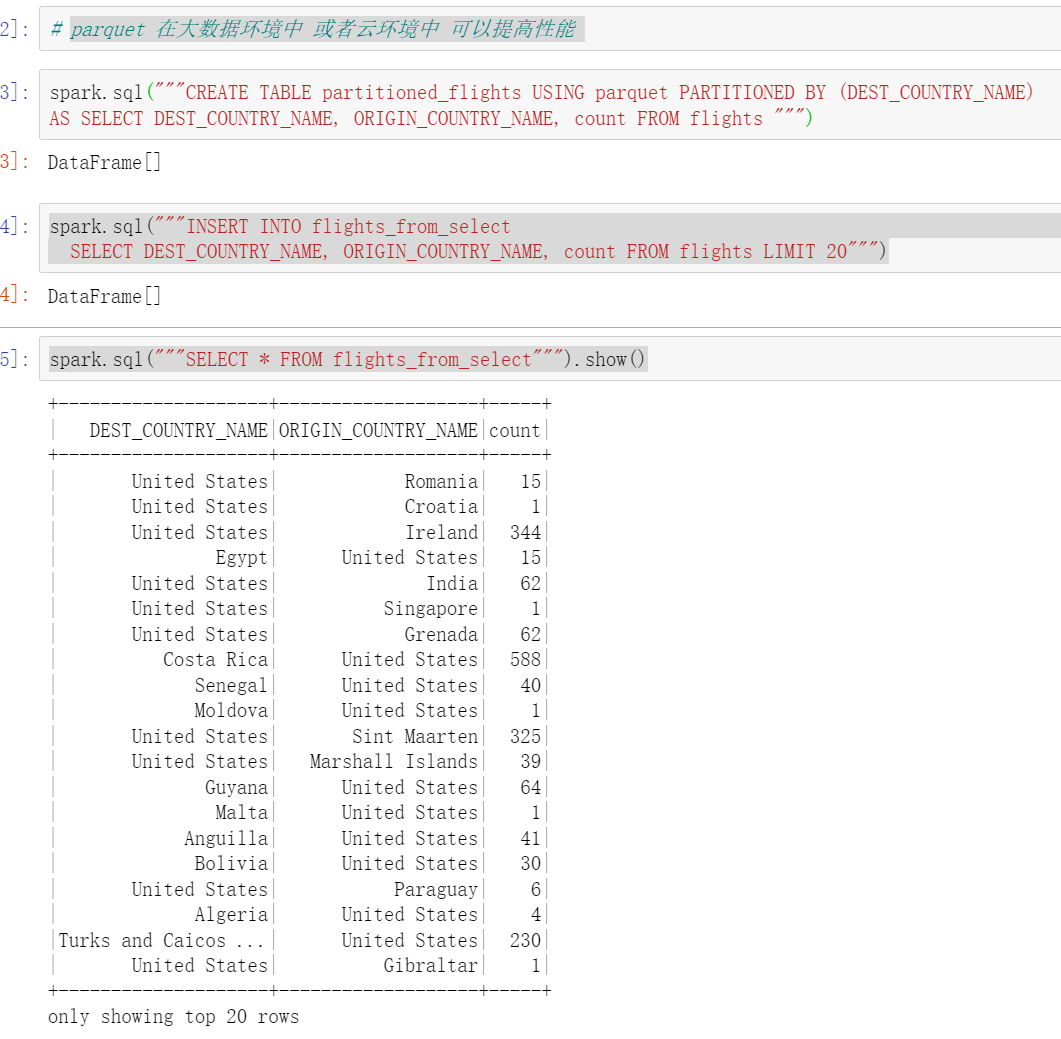
spark can support a variety of formats, such as CSV, JSON and many other data formats. It is common to use parquet in big data environment. Parquet can improve performance in big data environment or cloud environment. Performance will not be improved on a single machine. Multiple machines can be stored or read together in a cloud environment.

spark.sql("""CREATE TABLE flights_from_select USING parquet AS SELECT * FROM flights""")

#Create table structure
spark.sql("""CREATE TABLE partitioned_flights USING parquet PARTITIONED BY (DEST_COUNTRY_NAME)
AS SELECT DEST_COUNTRY_NAME, ORIGIN_COUNTRY_NAME, count FROM flights """)
#insert data
spark.sql("""INSERT INTO flights_from_select
  SELECT DEST_COUNTRY_NAME, ORIGIN_COUNTRY_NAME, count FROM flights LIMIT 20""")
#query
spark.sql("""SELECT * FROM flights_from_select""").show()

#Inserts a code block into the specified partition. PARTITION (DEST_COUNTRY_NAME="UNITED STATES") stands for inserting the specified partition
spark.sql("""INSERT INTO partitioned_flights
  PARTITION (DEST_COUNTRY_NAME="UNITED STATES")
  SELECT count, ORIGIN_COUNTRY_NAME FROM flights
  WHERE DEST_COUNTRY_NAME='United States' LIMIT 12
""")

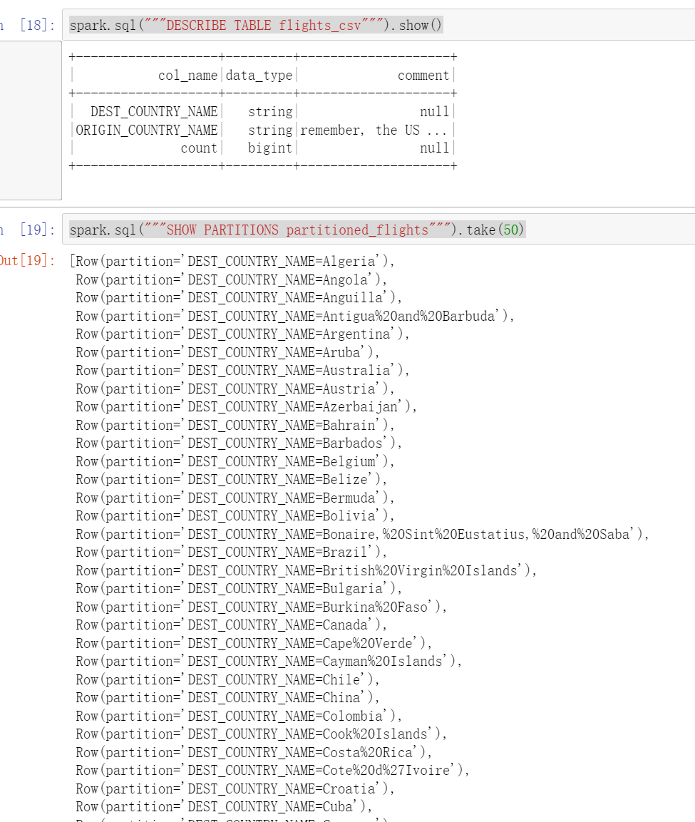
spark.sql("""DESCRIBE TABLE flights_csv""").show()
spark.sql("""SHOW PARTITIONS partitioned_flights""").take(50)

Cache accelerator – speed up data reading
spark.sql("""CACHE TABLE flights""")
spark.sql("""select * from flights""").show(5)
spark.sql("""UNCACHE TABLE flights""")

The fifth section uses spark for machine learning data mining

Infer how old you are, how many years you work, and how much you get.

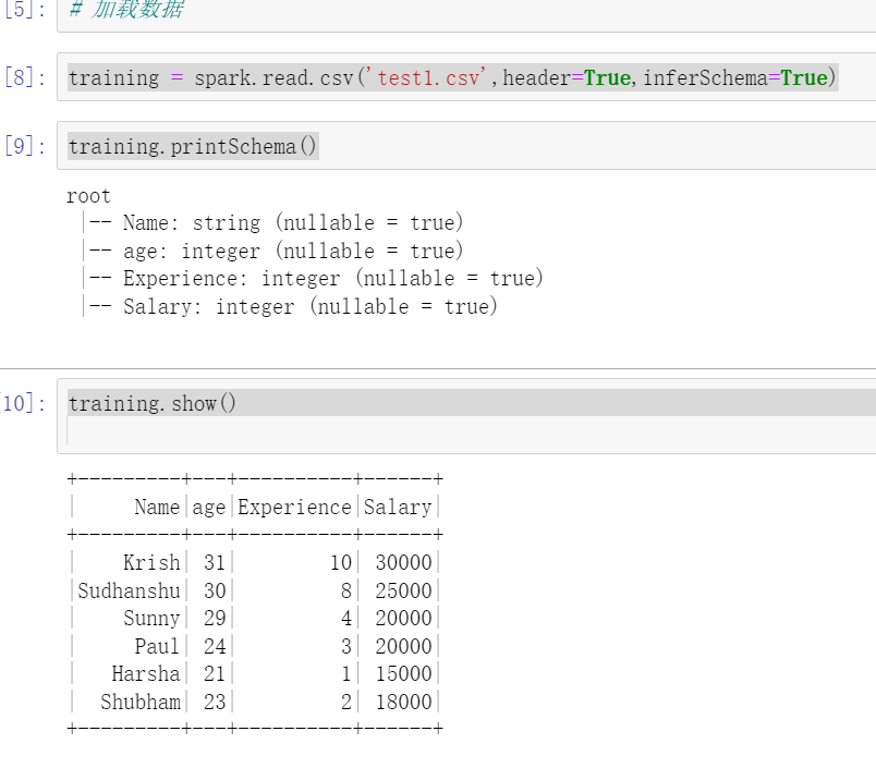
Load data

import findspark
findspark.init()
from pyspark.sql import SparkSession
spark=SparkSession.builder.appName('ML').getOrCreate()
training = spark.read.csv('test1.csv',header=True,inferSchema=True)
training.show()

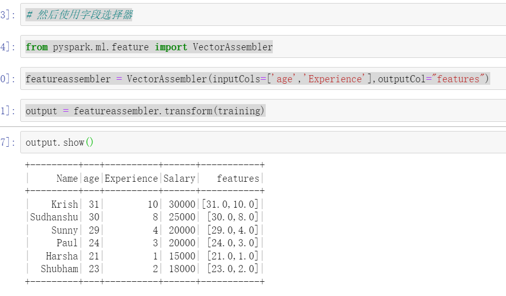
Use the field selector to select the field VectorAssembler

from pyspark.ml.feature import VectorAssembler
featureassembler = VectorAssembler(inputCols=['age','Experience'],outputCol="features")
output = featureassembler.transform(training)

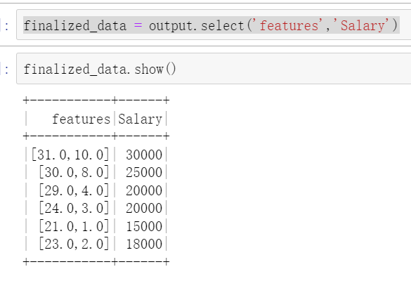
finalized_data = output.select('features','Salary')

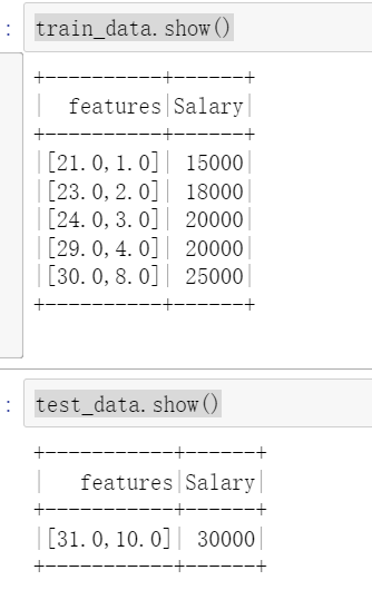
Import the linear regression model and split the data

from pyspark.ml.regression import LinearRegression
# Split the data into training data and test data 
train_data,test_data=finalized_data.randomSplit([0.75,0.25])
train_data.show()
test_data.show()

Create model

 regressor=LinearRegression(featuresCol='features',labelCol='Salary')
 regressor=regressor.fit(train_data)
 regressor.coefficients
 regressor.intercept 

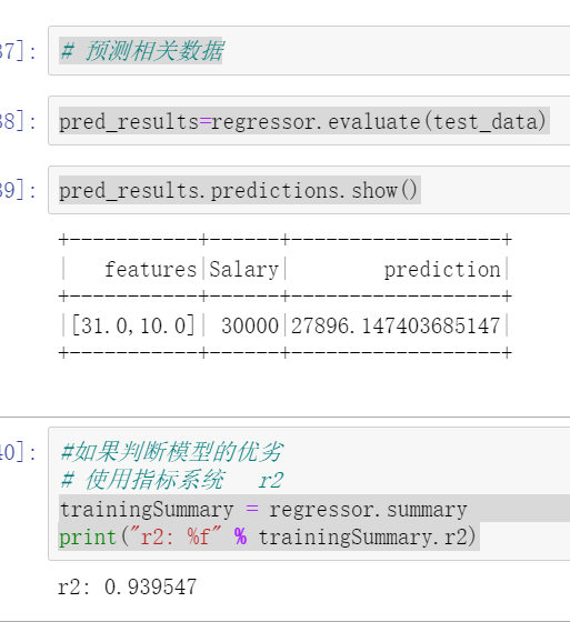
Use the test set to predict the relevant data and judge the advantages and disadvantages of the model

# Forecast related data
pred_results=regressor.evaluate(test_data)
pred_results.predictions.show()

#If you judge the advantages and disadvantages of the model
#Use indicator system r2

trainingSummary = regressor.summary
print("r2: %f" % trainingSummary.r2)