definition
Let's take a look at the example of playing cricket. Suppose you win a game today, it means a successful event. You played another game, but you lost. If you win a game today, it doesn't mean you will win tomorrow. Let's assign a random variable x to represent the number of wins. What is the possible value of X? It can be any value, depending on how many times you flip a coin.
There are only two possible outcomes, success and failure. Therefore, the probability of success = 0.5, and the probability of failure can be easily calculated: q = p – 1 = 0.5.
Binomial distribution is a distribution with only two possible outcomes, such as success or failure, gain or loss, win or lose. The probability of success and failure in each attempt is equal.
The results may not be equal. If the probability of success in the experiment is 0.2, the probability of failure can be easily calculated as q = 1 - 0.2 = 0.8.
Each attempt is independent, because the result of the previous throw cannot determine or affect the result of the current throw. An experiment with only two possible results and repeated N times is called binomial. The parameters of binomial distribution are n and p, where n is the total number of trials and p is the probability of success of each trial.
Based on the above description, the attributes of binomial distribution include:
- Each experiment is independent.
- There are only two possible outcomes in the experiment: success or failure.
- A total of n identical tests were performed.
- All trials have the same probability of success and failure. (the test is the same)
formula
𝑁⋅𝑝 represents the mean value of the distribution
-
PMF (probability quality function): it is the definition of discrete random variable Is the probability of discrete random variable in each specific value Generally speaking, this function is used to calculate the probability of each successful event result for a discrete probability event
-
Pdf (probability density function): it is the definition of continuous random variable Different from PMF, the value of PDF at a specific point is not the probability of that point. Continuous random probability events can only calculate the probability of events in a certain area by integrating this area Generally speaking, this probability density function is used to bring the critical points (maximum and minimum) of the interval where the probability is required into the integral Is the probability of the interval
TypeError: bar() missing 1 required positional argument: 'x'
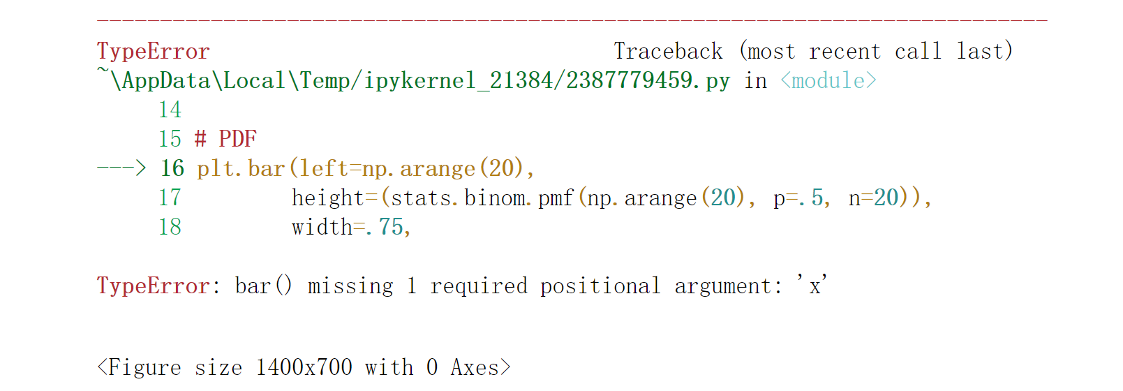
Change left to x:
plt.bar(left=np.arange(20),
height=(stats.binom.pmf(np.arange(20), p=.5, n=20)),
width=.75,
alpha=0.75
)
plt.bar(x=np.arange(20),
height=(stats.binom.pmf(np.arange(20), p=.5, n=20)),
width=.75,
alpha=0.75
)
# IMPORTS
import numpy as np
import scipy.stats as stats
import matplotlib.pyplot as plt
import matplotlib.style as style
from IPython.core.display import HTML

# PLOTTING CONFIG
%matplotlib inline
style.use('fivethirtyeight')
plt.rcParams["figure.figsize"] = (14, 7)

plt.figure(dpi=100)

# PDF
plt.bar(x=np.arange(20),
        height=(stats.binom.pmf(np.arange(20), p=.5, n=20)),
        width=.75,
        alpha=0.75
       )
# CDF
plt.plot(np.arange(20),
         stats.binom.cdf(np.arange(20), p=.5, n=20),
         color="#fc4f30",
        )

# LEGEND
plt.text(x=4.5, y=.7, s="pmf (normed)", alpha=.75, weight="bold", color="#008fd5")
plt.text(x=14.5, y=.9, s="cdf", alpha=.75, weight="bold", color="#fc4f30")

# TICKS
plt.xticks(range(21)[::2])
plt.tick_params(axis = 'both', which = 'major', labelsize = 18)
plt.axhline(y = 0.005, color = 'black', linewidth = 1.3, alpha = .7)

# TITLE, SUBTITLE & FOOTER
plt.text(x = -2.5, y = 1.25, s = "Binomial Distribution - Overview",
               fontsize = 26, weight = 'bold', alpha = .75)
plt.text(x = -2.5, y = 1.1,
         s = 'Depicted below are the normed probability mass function (pmf) and the cumulative density\nfunction (cdf) of a Binomial distributed random variable $ y \sim Binom(N, p) $, given $ N = 20$ and $p =0.5 $.',
         fontsize = 19, alpha = .85)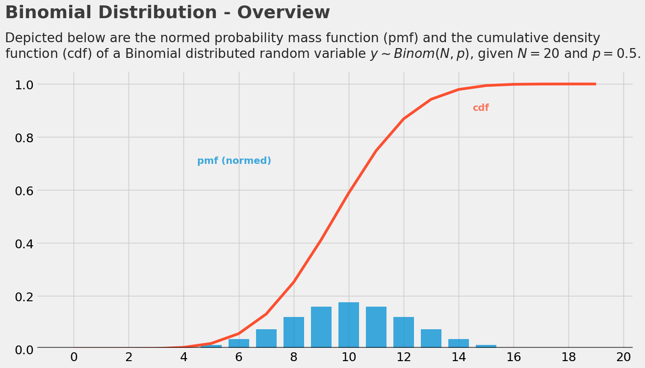
The impact on the results after changing the P value is shown in the following figure:
plt.figure(dpi=100)

# PDF P = .2
plt.scatter(np.arange(21),
            (stats.binom.pmf(np.arange(21), p=.2, n=20)),
            alpha=0.75,
            s=100
       )
plt.plot(np.arange(21),
         (stats.binom.pmf(np.arange(21), p=.2, n=20)),
         alpha=0.75,
        )

# PDF P = .5
plt.scatter(np.arange(21),
            (stats.binom.pmf(np.arange(21), p=.5, n=20)),
            alpha=0.75,
            s=100
       )
plt.plot(np.arange(21),
         (stats.binom.pmf(np.arange(21), p=.5, n=20)),
         alpha=0.75,
        )

# PDF P = .9
plt.scatter(np.arange(21),
            (stats.binom.pmf(np.arange(21), p=.9, n=20)),
            alpha=0.75,
            s=100
       )
plt.plot(np.arange(21),
         (stats.binom.pmf(np.arange(21), p=.9, n=20)),
         alpha=0.75,
        )

# LEGEND
plt.text(x=3.5, y=.075, s="$p = 0.2$", alpha=.75, weight="bold", color="#008fd5")
plt.text(x=9.5, y=.075, s="$p = 0.5$", alpha=.75, weight="bold", color="#fc4f30")
plt.text(x=17.5, y=.075, s="$p = 0.9$", alpha=.75, weight="bold", color="#e5ae38")

# TICKS
plt.xticks(range(21)[::2])
plt.tick_params(axis = 'both', which = 'major', labelsize = 18)
plt.axhline(y = 0, color = 'black', linewidth = 1.3, alpha = .7)

# TITLE, SUBTITLE & FOOTER
plt.text(x = -2.5, y = .37, s = "Binomial Distribution - $p$",
               fontsize = 26, weight = 'bold', alpha = .75)
plt.text(x = -2.5, y = .32,
         s = 'Depicted below are three Binomial distributed random variables with varying $p $. As one can see\nthe parameter $p$ shifts and skews the distribution.',
         fontsize = 19, alpha = .85)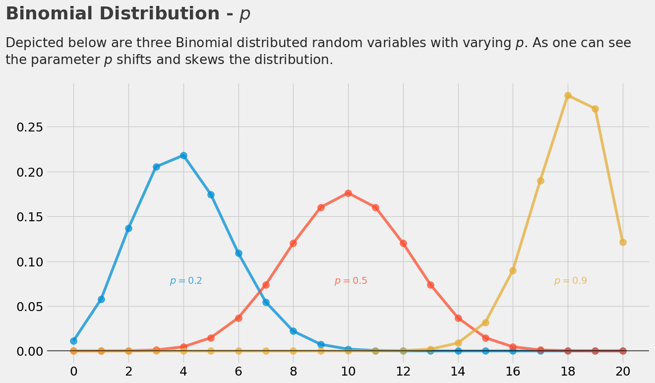
The effect of changing the N value on the results is as follows:
plt.figure(dpi=100)

# PDF N = 10
plt.scatter(np.arange(11),
            (stats.binom.pmf(np.arange(11), p=.5, n=10)),
            alpha=0.75,
            s=100
       )
plt.plot(np.arange(11),
         (stats.binom.pmf(np.arange(11), p=.5, n=10)),
         alpha=0.75,
        )

# PDF N = 15
plt.scatter(np.arange(16),
            (stats.binom.pmf(np.arange(16), p=.5, n=15)),
            alpha=0.75,
            s=100
       )
plt.plot(np.arange(16),
         (stats.binom.pmf(np.arange(16), p=.5, n=15)),
         alpha=0.75,
        )

# PDF N = 20
plt.scatter(np.arange(21),
            (stats.binom.pmf(np.arange(21), p=.5, n=20)),
            alpha=0.75,
            s=100
       )
plt.plot(np.arange(21),
         (stats.binom.pmf(np.arange(21), p=.5, n=20)),
         alpha=0.75,
        )

# LEGEND
plt.text(x=6, y=.225, s="$N = 10$", alpha=.75, weight="bold", color="#008fd5")
plt.text(x=8.5, y=.2, s="$N = 15$", alpha=.75, weight="bold", color="#fc4f30")
plt.text(x=11, y=.175, s="$N = 20$", alpha=.75, weight="bold", color="#e5ae38")

# TICKS
plt.xticks(range(21)[::2])
plt.tick_params(axis = 'both', which = 'major', labelsize = 18)
plt.axhline(y = 0, color = 'black', linewidth = 1.3, alpha = .7)

# TITLE, SUBTITLE & FOOTER
plt.text(x = -2.5, y = .31, s = "Binomial Distribution - $N$",
               fontsize = 26, weight = 'bold', alpha = .75)
plt.text(x = -2.5, y = .27,
         s = 'Depicted below are three Binomial distributed random variables with varying $N$. As one can see\nthe parameter $N$ streches the distribution (the larger $N$ the flatter the distribution).',
         fontsize = 19, alpha = .85)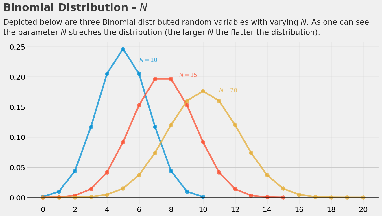
Random variables can also be constructed:
import numpy as np
from scipy.stats import binom

# draw a single sample
np.random.seed(42)
print(binom.rvs(p=0.3, n=10), end="\n\n")

# draw 10 samples
print(binom.rvs(p=0.3, n=10, size=10), end="\n\n")
2

[5 4 3 2 2 1 5 3 4 0]
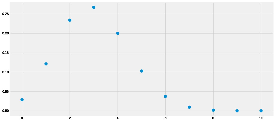
Calculate the probability of the probability mass function:
from scipy.stats import binom

# additional imports for plotting purpose
import numpy as np
import matplotlib.pyplot as plt
%matplotlib inline
plt.rcParams["figure.figsize"] = (14,7)

# likelihood of x and y
x = 1
y = 7
print("pmf(X=1) = {}\npmf(X=7) = {}".format(binom.pmf(k=x, p=0.3, n=10), binom.pmf(k=y, p=0.3, n=10)))

# continuous pdf for the plot
x_s = np.arange(11)
y_s = binom.pmf(k=x_s, p=0.3, n=10)
plt.scatter(x_s, y_s, s=100);
pmf(X=1) = 0.12106082099999989 pmf(X=7) = 0.009001691999999992
Calculate the probability of cumulative probability density function:
from scipy.stats import binom

# probability of x less or equal 0.3
print("P(X <=3) = {}".format(binom.cdf(k=3, p=0.3, n=10)))

# probability of x in [-0.2, +0.2]
print("P(2 < X <= 8) = {}".format(binom.cdf(k=8, p=0.3, n=10) - binom.cdf(k=2, p=0.3, n=10)))
P(X <=3) = 0.6496107183999998 P(2 < X <= 8) = 0.6170735276999999