preface

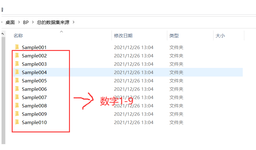
This program can identify the numbers 1-9. A total of 270 pictures in the training set are used for training, that is, 30 pictures for each number are used for training. Finally, in the test set, 10 pieces of each number, that is, 90 pieces, were found for accurate identification. Note this article is reproduced in:( Recognition of handwritten digits by BP neural network (item analysis and code) , the original code can not be run directly, so this paper provides the data set and test set based on it.

1: Data set source

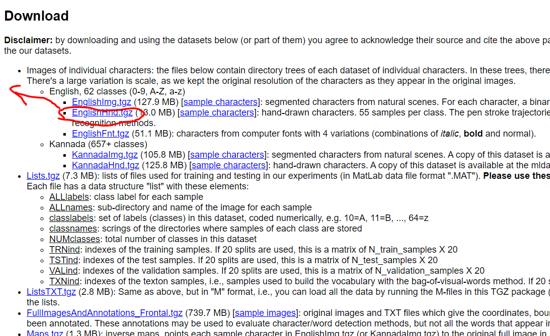
Prepare the training set and test set. Libraries used are from http://www.ee.surrey.ac.uk/CVSSP/demos/chars74k/#download
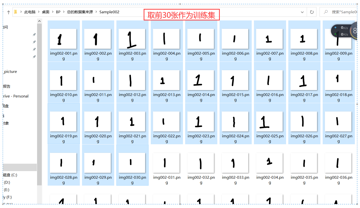
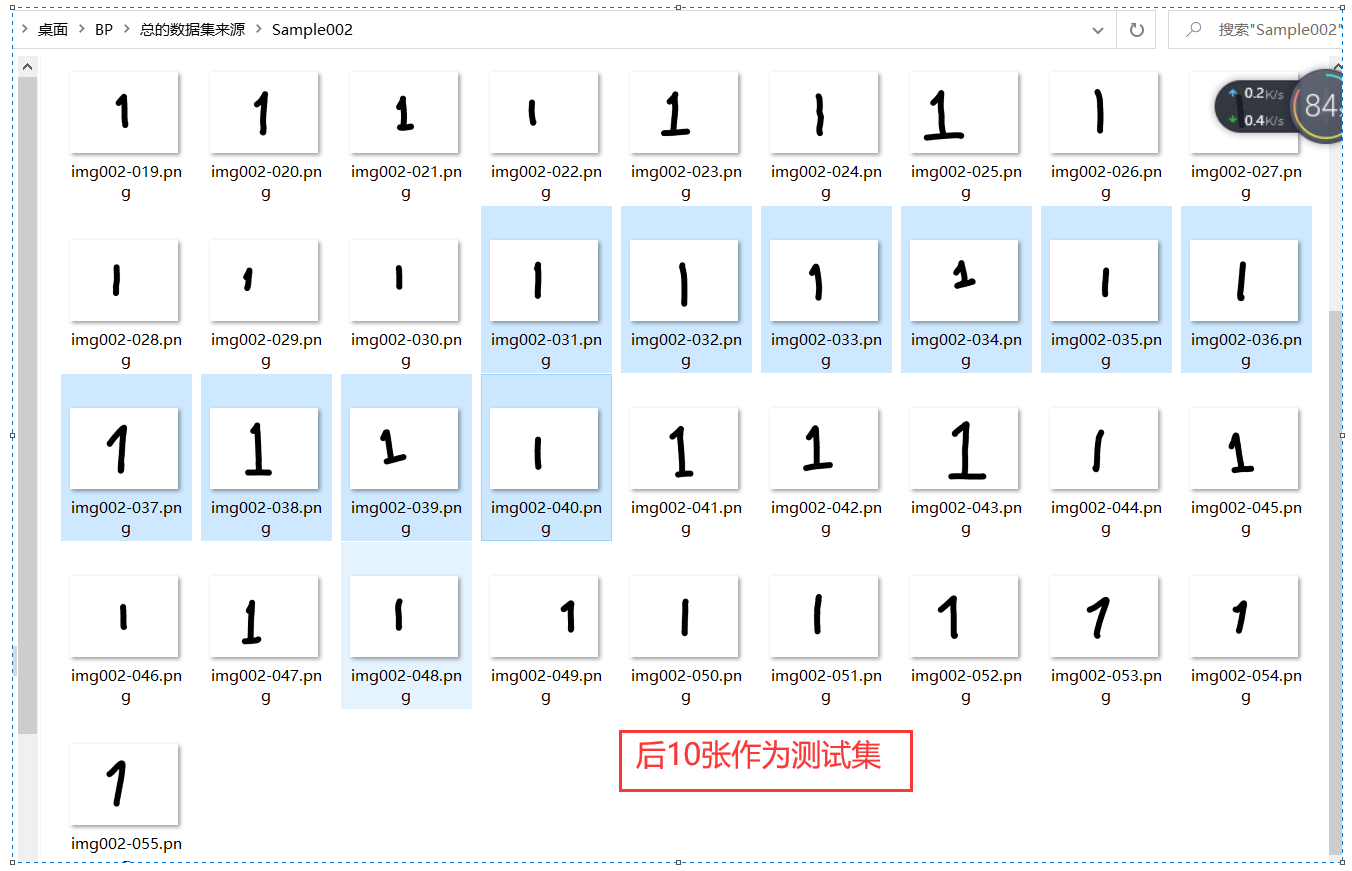
Use englishhnd Tgz library, select the first 30 for each number as training, and then take another 10 as test.

Figure 1

Figure 2

Figure 3

Figure 4

Figure 5

2: Principle

(1) Traditional neural network in vernacular
First, let's look at the basic unit of neural network - single neuron:

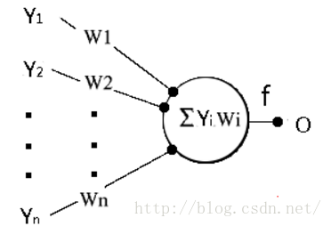
The circle in the figure represents a neuron. We know that a neuron receives stimuli from adjacent neurons. Neurons accumulate these stimuli with different weights, generate their own stimuli at a certain time, and transmit them to some adjacent neurons. The countless neurons working in this way constitute the human brain's perception of the outside world. The mechanism of human brain's learning of the world is to adjust the weight of these adjacent connected neurons.
In the figure, the stimulus transmitted by the surrounding neurons is represented as Y, and the weight is represented as W. the stimulus obtained by the round neurons is that all stimuli are accumulated according to the weight, i.e
At the same time, as a part of the network, this neuron, like other neurons, needs to spread stimulation signals outward, but it does not spread s directly, but spread an f(s). Why? In fact, it doesn't matter. We'll analyze it later. The name of f(s) is "activation function", and the commonly used functions are as follows:

Well, if there's no problem here, congratulations. You've started. Now we connect the basic units one by one to form our final neural network. The traditional neural network structure is shown in the figure below

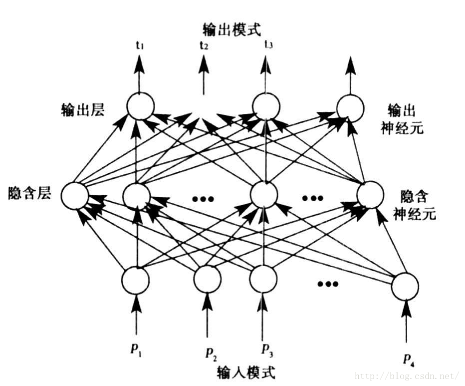
Do you think it's messy? Don't worry. Let's look at it bit by bit and dissect it from the whole to the details. Firstly, on the whole, its structure is divided into three parts: input layer, hidden layer and output layer. Generally, there is one input layer and one output layer, and several hidden layers. One is drawn in the figure. In detail, in the connection structure, each neuron in the latter layer is connected by all neurons in the previous layer.
The handwritten numeral recognition experiment uses a three-layer neural network structure, that is, there is only one hidden layer, which is explained below.
The following describes the representation and relationship of each layer:
Input layer: X=(x1,x2,x3... xn)
Hidden layer: Y=(y1,y2,y3... ym)
Output layer: O=(o1,o2,o3... or)

Two weights:
Weight from input layer to hidden layer: V=(V1,V2,V3... Vm), Vj is a column vector, indicating that all neurons in the input layer are weighted by Vj to obtain the j th neuron in the hidden layer
Weight from hidden layer to output layer: W=(W1,W2,W3... Wr), Wk is a column vector, indicating that all neurons in the hidden layer are weighted by Wk to obtain the kth neuron in the output layer

According to the above-mentioned stimulation afferent and stimulation efferent of a single neuron, I believe that many people should have obtained the relationship between the following layers:

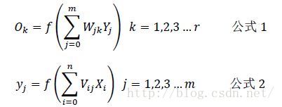
Here, the working process of neural network is clearer. For example, suppose that the input is an image, 16X16 in size, converted into a two-dimensional gray value matrix, and then each row is spliced at the end of the previous row to form a 1x256 row vector as the input of the input layer, that is, X. next, the hidden layer can be calculated according to formula 2, and then the output layer can be calculated according to Formula 1, The output of the output layer is obtained. In this handwritten numeral recognition project, the picture input I used was 16x16, so there were 256 neurons in the input layer, 64 neurons in the hidden layer, and 10 neurons in the final output layer. Why 10? There are 10 numbers from 0 to 9. It is expected that, for example, if you input an image with the number 1, the output at the output end is {1 0 0 0 0 0 0 0 0 0 0 0 0 0 0 0 0 0 0 0 0 0 0 0 0 0 0 0 0 0 0 0 0 0 0 0 0 0 0 0 0 0 0 0 0 0 0 0 0 0 0 0 0 0 0 0 0 0 0 0 0 0 0 0 0 0 0 0 0 0 0 0 0 0 0 0 0 0 0 0 0 0 0 0 0 0 0 0 0 0 0 0 0 0 0 0 0 0 0 0 0 0 0 0 0 0 0 0 0 0 0 0 0 0 0 0 0 0 0 0 0 0 0 0 0, The number on the image can be recognized only by judging the position of the maximum value.

So far, we have understood the structure of the whole network and the specific process of forward work. It can be said that we have understood neural networks by 50%. Why only 50%? Think about it carefully. I believe you will find that we don't know two very important quantities in the network, namely weight matrix W and V.

How to find w and V? An algorithm is used here, that is, error back propagation algorithm (BP algorithm for short). It's very obscure. Let's translate adult words. Let's take a look at the working process of the algorithm. First, initialize the values of W and V randomly, and then substitute some pictures for calculation to obtain an output. Of course, since the parameters of W and V are not exactly perfect, the output will not be like {1 0 0 0 0 0 0 0 0 0 0 0 0 0 0 0 0 0 0 0 0 0 0 0 0 0 0 0 0 0 0 0 0 0 0 0 0 0 0 0 0 0 0 0 0 0 0 0 0 0 0 0 0 0 0 0 0 0 0 0 0 0 0 0 0 0 0 0 0 0 0 0 0 0 0 0 0 0 0 0, The corrected W and V can make the output closer to the ideal output, which is the meaning of the so-called "error back propagation". After correction once, replace some other pictures. The output is a little closer to the ideal output. We continue to calculate the error, and then correct the values of W and V. after many iterative calculations, Finally, the perfect W and V matrices are obtained by multiple corrections, which can make the output very close to the ideal output. So far, our work completion is 100%. This idea of calculating the error at the output and adjusting it according to the error. Students who learn automation or have been in contact with smart car competitions such as Freescale should have a deep experience, which is very similar to PID automatic control algorithm.

The following is a mathematical derivation. How to specifically adjust the values of W and V and how much to adjust the error between the actual output and the ideal output. As mentioned above, if you don't understand it for the time being, you can skip the derivation and see the final conclusion. Finally, you can practice it with the code, have a deeper experience and understand it slowly.

(2) Mathematical derivation of back propagation algorithm
Ideal output of output layer: d=(d1,d2,d3... dr), such as {1 0 0 0 0 0 0 0 0 0 0 0 0 0 0 0 0 0 0 0 0 0 0 0 0 0 0 0 0 0 0 0 0 0 0 0 0 0 0 0 0 0 0 0 0 0 0 0 0 0 0 0 0 0 0 0 0 0 0 0 0 0 0 0 0 0 0 0 0 0 0 0 0
Assuming that the difference between the actual output and the ideal output is E, it is obvious that w is a function of input X, weights w and V, and output O. To correct W, you need to know the specific correction increment Δ W. In the case of discretization, the differential increment can be characterized, and the following can be obtained:


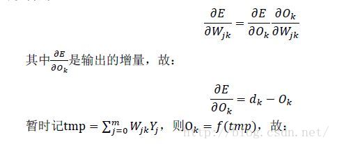
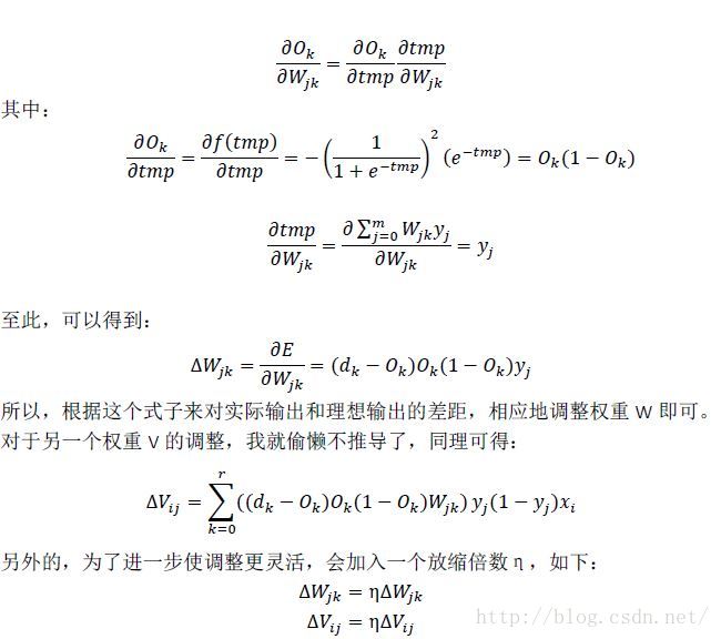
So, change η The magnitude of each adjustment can be changed, η If it is large, the adjustment is faster, and if it is small, the adjustment is slow, but if it is too large, it is easy to cause oscillation, which is the same as the proportional coefficient P in PID. commonly η The size of requires multiple attempts to find the appropriate value.

Well, that's the end of the neural network. The following is a minor content. As we said above, we adjust the weights W and V through continuous iteration. So how to measure whether the iteration can stop. A natural idea is to judge whether the output of each time is close enough to the ideal output, so we can use the method of calculating the vector distance, which is the same as the mean square deviation, as follows:

In this way, the main s is small enough for the iteration to end.

3: Code part

train.m Code of

V=double(rand(256,64));
W=double(rand(64,10));
delta_V=double(rand(256,64));
delta_W=double(rand(64,10));

yita=0.2;%Scaling factor, some articles call learning rate
yita1=0.05;%I add my own parameters and scale the independent variables of the activation function to prevent the input from entering the saturation area of the function. You can get rid of them and experience the changes
train_number=9;%How many numbers are there in the training sample, 9 in total, without 0
train_num=30;%In the training sample, how many maps are there for each number, a total of 100
x=double(zeros(1,256));%Input layer
y=double(zeros(1,64));%The middle layer is also a hidden layer
output=double(zeros(1,10));%Output layer
tar_output=double(zeros(1,10));%Target output, i.e. ideal output
delta=double(zeros(1,10));%An intermediate variable that can be ignored

%Record the total mean square deviation for drawing
s_record=1:400;
tic %time
for train_control_num=1:400   %The number of training times is controlled. At the end of parameter adjustment, it is found that there are more than 1000 times, about 400 times is enough
    s=0;
    %Read the picture and input the network
    for number=2:(1+train_number) %train_number=10 Because the file name of the picture is from img002 Beginning,So this is 2
        ReadDir=['C:\Users\Lenovo\Desktop\BP\train_picture\'];%Path to read samples
        for num=1:train_num  %How many sheets are controlled  train_num=30
            if number~=10  %When the file name of the picture reaches 10, the name will change, so it is discussed here
                photo_name=['img00',num2str(number) ,'-',num2str(num,'%03d'),'.png'];%The picture name is spliced
                photo_index=[ReadDir,photo_name];%Path plus picture name to get the total picture index
                photo_matrix=imread(photo_index);%use imread Get image matrix
                photo_matrix=rgb2gray(photo_matrix);
                photo_matrix=imresize(photo_matrix,[16,16]);
                photo_matrix=uint8(photo_matrix<=230);%Binarization, black is 1
                
                tmp=photo_matrix';
                tmp=tmp(:);%In the above two steps, the image two-dimensional matrix is transformed into column vector, 256 dimensions, as input
                %Calculation input layer input
                x=double(tmp');%Convert to line vector because of the input layer X Is a row vector and is converted to a floating point number
                %Get hidden layer input
                y0=x*V;
                %activation
                y=1./(1+exp(-y0*yita1));
                %Get output layer input
                output0=y*W;
                % lf=lf+1;Reference data used to see where the error is
                output=1./(1+exp(-output0*yita1));
                %Calculate expected output
                tar_output=double(zeros(1,10));
                tar_output(number)=1.0;
                %calculation error
                %Calculated according to the formula W and V To avoid the use of for The cycle comparison takes time. The following uses direct matrix multiplication, which is more efficient
                delta=(tar_output-output).*output.*(1-output);
                delta_W=yita*repmat(y',1,10).*repmat(delta,64,1);
                tmp=sum((W.*repmat(delta,64,1))');
                tmp=tmp.*y.*(1-y);
                delta_V=yita*repmat(x',1,64).*repmat(tmp,256,1);
                %Calculate mean square deviation
                s=s+sum((tar_output-output).*(tar_output-output))/10;
                %Update weight
                W=W+delta_W;
                V=V+delta_V;
            else
                photo_name=['img0',num2str(number) ,'-',num2str(num,'%03d'),'.png'];%Picture name
                photo_index=[ReadDir,photo_name];%Path plus picture name to get the total picture index
                photo_matrix=imread(photo_index);%use imread Get image matrix
                photo_matrix=rgb2gray(photo_matrix);
                photo_matrix=imresize(photo_matrix,[16,16]);
                photo_matrix=uint8(photo_matrix<=230);%Binarization, black is 1
                
                tmp=photo_matrix';
                tmp=tmp(:);%In the above two steps, the image two-dimensional matrix is transformed into column vector, 256 dimensions, as input
                %Calculation input layer input
                x=double(tmp');%Convert to line vector because of the input layer X Is a row vector and is converted to a floating point number
                %Get hidden layer input
                y0=x*V;
                %activation
                y=1./(1+exp(-y0*yita1));
                %Get output layer input
                output0=y*W;
                % lf=lf+1;Reference data used to see where the error is
                output=1./(1+exp(-output0*yita1));
                %Calculate expected output
                tar_output=double(zeros(1,10));
                tar_output(number)=1.0;
                %calculation error
                %Calculated according to the formula W and V To avoid the use of for The cycle comparison takes time. The following uses direct matrix multiplication, which is more efficient
                delta=(tar_output-output).*output.*(1-output);
                delta_W=yita*repmat(y',1,10).*repmat(delta,64,1);
                tmp=sum((W.*repmat(delta,64,1))');
                tmp=tmp.*y.*(1-y);
                delta_V=yita*repmat(x',1,64).*repmat(tmp,256,1);
                %Calculate mean square deviation
                s=s+sum((tar_output-output).*(tar_output-output))/10;
                %Update weight
                W=W+delta_W;
                V=V+delta_V;
            end
        end
    end
    s=s/train_number/train_num;  %Without semicolon, output error at any time and watch convergence
    train_control_num           %Without semicolon, output the number of iterations at any time and watch the running state
    s_record(train_control_num)=s;%record
end
toc %Timing end
plot(1:400,s_record);
save result W V yita1; %preservation W V yita1 And name it result2 

test.m Code of

correct_num=0;%Record the correct quantity
incorrect_num=0;%Number of recorded errors
test_number=9;%In the test set, how many numbers are there, 9, no 0
test_num=10;%How many numbers are there in the test set? The maximum number is 100
%load W;%%From previous training W After saving, you can load it directly
%load V;
%load yita1;

%Record time
tic %Timing start
for number=2:(1+test_number)
    ReadDir=['C:\Users\Lenovo\Desktop\BP\test_picture\'];
    for num=31:(30+test_num)  %How many sheets are controlled
        if number~=10
            photo_name=['img00',num2str(number) ,'-',num2str(num,'%03d'),'.png'];%Picture name
            photo_index=[ReadDir,photo_name];%Path plus picture name to get the total picture index
            photo_matrix=imread(photo_index);%use imread Get image matrix
            photo_matrix=rgb2gray(photo_matrix);
            photo_matrix=imresize(photo_matrix,[16,16]);%Size change
            photo_matrix=uint8(photo_matrix<=230);%Binarization, black is 1
            %Row vector
            tmp=photo_matrix';
            tmp=tmp(:);
            %Calculation input layer input
            x=double(tmp');
            %Get hidden layer input
            y0=x*V;
            %activation
            y=1./(1+exp(-y0*yita1));
            %Get output layer input
            o0=y*W;
            o=1./(1+exp(-o0*yita1));
            %The largest output is the recognized number
            [o,index]=sort(o);
            if index(10)==number
                correct_num=correct_num+1
            else
                incorrect_num=incorrect_num+1;
                %The display of unsuccessful numbers will take more time
%                      figure(incorrect_num)
%                      imshow((1-photo_matrix)*255);
%                      title(num2str(number));
            end
        else
            photo_name=['img0',num2str(number) ,'-',num2str(num,'%03d'),'.png'];%Picture name
            photo_index=[ReadDir,photo_name];%Path plus picture name to get the total picture index
            photo_matrix=imread(photo_index);%use imread Get image matrix
            photo_matrix=rgb2gray(photo_matrix);
            photo_matrix=imresize(photo_matrix,[16,16]);%Size change
            photo_matrix=uint8(photo_matrix<=230);%Binarization, black is 1
            %Row vector
            tmp=photo_matrix';
            tmp=tmp(:);
            %Calculation input layer input
            x=double(tmp');
            %Get hidden layer input
            y0=x*V;
            %activation
            y=1./(1+exp(-y0*yita1));
            %Get output layer input
            o0=y*W;
            o=1./(1+exp(-o0*yita1));
            %The largest output is the recognized number
            [o,index]=sort(o);
            if index(10)==number
                correct_num=correct_num+1
            else
                incorrect_num=incorrect_num+1;
                %The display of unsuccessful numbers will take more time
                %     figure(incorrect_num)
                %     imshow((1-photo_matrix)*255);
                %     title(num2str(number));
            end
        end
    end
end
correct_rate=correct_num/test_number/test_num
toc %Timing end
save result2 correct_rate; %Save the result of recognition rate and name it as result2 

Supplementary, in test In M, there are the following lines of code, which are explained here:

o=1./(1+exp(-o0*yita1));
            %The largest output is the recognized number
            [o,index]=sort(o);
            if index(10)==number
                correct_num=correct_num+1
            else

Look at the picture: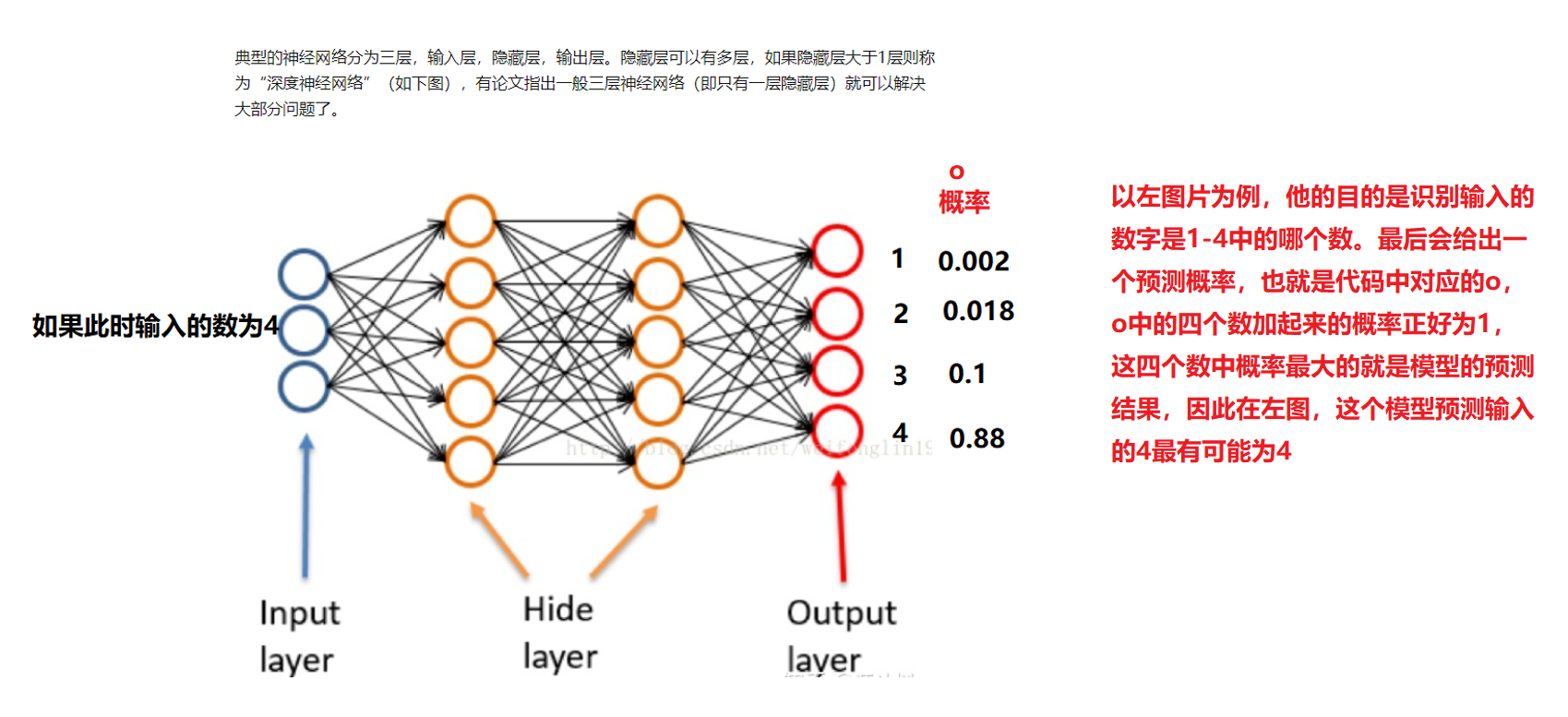

Figure 6

In O, there are 10 outputs, and we want to predict the 9 numbers from 1 to 9 (forget 0 for the time being), then the probability of these numbers will be given in O, and the prediction result is the one with the largest probability. [o,index]=sort(o); It means sorting the probability in O, and index is the sorted index,
if index(10)==number means that if the index of the largest number in the index is exactly equal to the number entered at this time, it means that the prediction is correct. It's a little difficult to understand. Look at the figure below.

Figure 7