Note: Mr. Liu's notes on the content of algorithm design and analysis course this semester

People who have to stick to it until the end feel great
Besides, PPT is not well understood by the teacher behind the teacher. Of course, it may be because I am always distracted and make complaints about it. 🤔

Branch gauge

Loading problem analysis 🚩

Breadth first search

• Use queue
  
• Use priority queue:

cw: current weight, r: remaining weight, improvement: priority queue
Design key value key=cw+r, select the extension node according to the key value
Constraint cw ≤ c, node record: (key;cw) / / omit the layer number
The blue node does not need to be extended: key is the upper bound of cw on the subtree / / contrast backtracking
It is also possible to prune using boundary conditions and updating the optimal value in advance

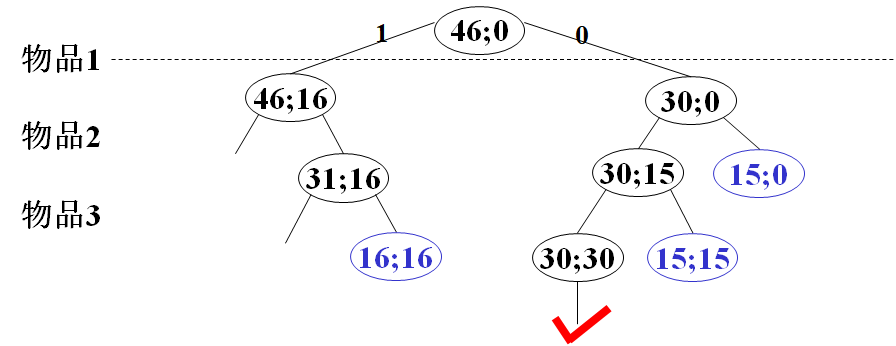
• Branch gauge

Branch and bound: upper bound key, lower bound bestw, key value key
cw, r, bestw, key = cw + r, t / / layer number
==Node record: (key; t, cw, r, bestw)==
Constraint: cw ≤ c + clearance: key > bestw + update in advance
End: T > n or queue empty or upper bound = lower bound

Summary: general steps of branch and gauge
Breadth first search
General process:

1. The initial root node is a live node (gray, in the queue), and other nodes are white
2. while(true)
3. Take a live node from the queue and set it as an extension node (red)
4. Set all children of the expansion node as live nodes (gray, in the queue),
5. Set expansion node as dead node (black)
   Live node fetching mode: first in first out queue or priority queue
   End method: the queue is empty or reaches the leaf node (design required)
   Nodes: four colors and three states
   There is only one extension node at any time

Dijkstra: priority queue or first in first out
Input: G=(V,E,w,s), w weight, s starting point;
Output: δ (s,·)

1. initial d[s]=0, other d[u]=INF,  
2.  S,Q empty, Q.add(s,0), 
3. When Q Non empty          //Q is the priority queue
4.    Q.delete(u), if uS, continue(),
5.    take u Add to S in, 
6.    arbitrarily v∈adj[u], slack(u,v), 
7.            if d[v]change, Q.add(v,d[v]) 
slack(u,v):  if d[v]>d[u]+w[u,v], be d[v]=d[u]+w[u,v]

Ah, ah, ah, ah, ah, ah, ah, ah, ah, ah, ah, ah, ah, ah, ah, ah, ah, ah, ah, ah, ah, ah, ah, ah, ah, ah, ah, ah, ah, ah, ah, ah, ah, ah, ah 😵🥴🧠

Summary
Backtracking: search solution space in depth first way
Branch and bound: search the solution space with breadth first or minimum cost
Regardless of pruning, the time complexity is O(|E|),
The space complexity is too different: O(h) vs O(|E|)
If you need to search the entire solution space, does branch and bound have any advantage?
Branch and bound is generally used to find an optimal solution and use priority queue
Upper bound, lower bound, key value It ends when you reach the nth floor
Lower bound: bestw, upper bound = key value = cw + remaining weight
Once the leaf node (r=0) is obtained, the upper bound = bestw=cw and the search is ended
Maintenance: upper bound, lower bound, key value, record information

I blew it up 🧨

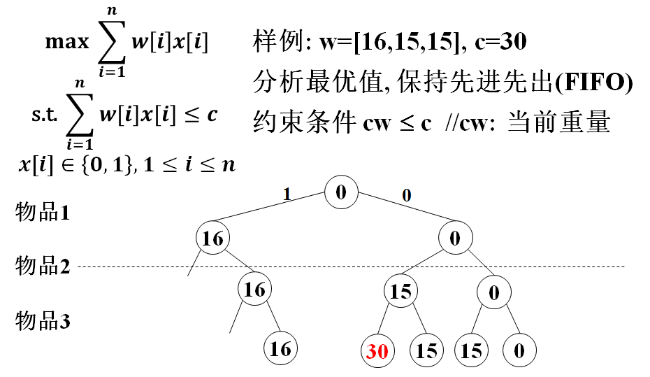
Loading problem

Branch and gauge design
Upper bound: key=cw+r, cw ≤ key of current node and its subtree nodes
Lower bound: bestw. You need to find a cw larger than bestw
Key value: key Take the live node with the largest key
Record information (t,cw,r) / / layer number, current weight, remaining weight
End when t > n: r=0, key=bestw=cw, and the remaining live node key is worthless
Find the optimal value, ignore the optimal solution, constraint conditions, bound conditions

upper bound key=cw+r, Lower bound bestw, Key value key, record(t,cw,r), Maximum heap
1. t=0, cw=0, bestw=0, r=sumi=1n w[i], key=r  //initial 
2. When t< n+1    //End when t=n+1
3. |   wt = cw + w[t], r1=r-w[t], ;
4. |   if wt ≤ c, if wt>bestw, be bestw=wt, 
5. |                     Q.add(wt+r1; t+1,wt,r1) 
6. |   if key > bestw, Q.add(cw+r1; t+1,cw,r1),   
7. |   Q.delete(key;t,cw,r) //Live node with maximum key value 

Maximum clique problem

Upper bound none, Lower bound bestn, Key value cn+n-t, record(t,cn,x) 
1. t=1, cn=0, bestn=0, x[1:n]=0,     //initial 
2. When t < n+1                          //When t=n+1, the search ends 
3. |   if vt And x[1:t-1]Existing in cn All points are connected, //constraint
4. |    |   x[t]=1, Q.add(cn+n-t+1; t+1,cn+1,x), x[t]=0 
5. |    |   if cn+1>bestn, bestn=cn+1 //Update the optimal value in advance 
6. |   if cn+n-t ≥ bestn, Q.add(cn+n-t; t+1,cn,x), //Gauge 
7. |   Q.delete( ; t,cn,x)         //Live node with maximum critical value 

Compare backtracking method with branch and bound method
Pruning functions can be shared
Can update the optimal value in time
Advantages of backtracking: less storage
Advantages of branch and bound: Live nodes can be freely selected as expansion nodes
Backtracking can be used to search for all optimal solutions
Branch and bound can be used to search for an optimal solution

Traveling salesman problem (TSP)

Branch and gauge design
It is currently set at the t-th floor
x[0:t]: the selected path from x[0] to x[t]
x[t+1:n-1]: remaining vertices
CC: cost of x [1: T]
bestc: current best cost (upper bound)
minout[t]: the minimum weight of the edge of vertex t
Rcost = sum of minout[x[i]] of x [t: n-1]
Key value: cc + rcost
Lower bound = critical value
Record (t, cc, rcost, x)

rcost=sumk=0n-1 minout[k]

1. t=0,cc=0,bestc=INF, rcost=sumk=0n-1 minout[k], x[0]=1
2. When t < n-1,     //When t=n-1, the search ends, priority queue, minimum heap
3.  |  if t = n-2 And feasible(Can you go back to 1), 
4.  |   | to update bestc, Q.add(cc; t+1,cc,0,x), continue()//Possible export 
5.  |  yes j = t : n-1, 
6.  |   | exchange x[t],x[j] 
7.  |   | if x[t-1],x[t]Edge, 
8.  |   |  | calculation cc, rcost,  if cc+rcost<bestc, Q.add(cc+rcost; t+1, cc,rcost,x) 
9.  |   | exchange x[t],x[j] 
10.|  Q.delete( ; t,cc,rcost,x)    //Live node with minimum critical value 

I will listen to the class next semester. I will listen to the class. I will listen to the class 🙍‍♀️

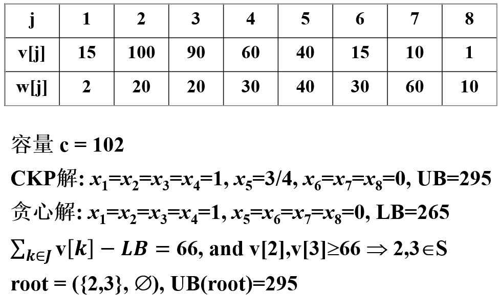
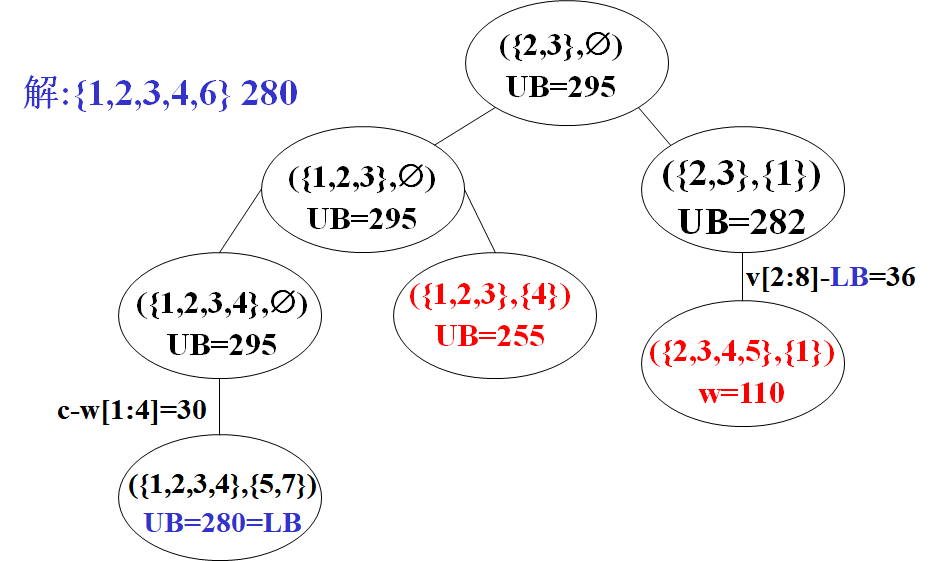
01 knapsack problem

Branch and gauge design
Upper bound: key=cv+r, cv ≤ key of current node and its subtree nodes
Lower bound: bestv. You need to find a cv larger than bestv
Key value: key Take the live node with the largest key
Record the information (t,cw,cv,r) / / layer number, current weight, current value and residual value
End when t > n: r=0, key=cv=bestv, and the remaining live node key is worthless
Find the optimal value, ignore the optimal solution, constraint conditions, bound conditions

upper bound key=cv+r, Lower bound bestv, Key value key, record(t,cw,cv,r), Maximum heap
1. t=0, cw=0, cv=0, bestv=0, r=sumi=1n v[i], key=r  
2. When t< n+1    //End when t=n+1
3. |   wt = cw + w[t], vt=cv+v[t], r1=r-v[t], ;
4. |   if wt ≤ c, if vt>bestv, be bestv=vt, 
5. |                     Q.add(vt+r1; t+1,wt,vt,r1) 
6. |   if key > bestv, Q.add(cw+r1; t+1,cw,cv,r1),   
7. |   Q.delete(key;t,cw,cv,r) //Live node with maximum key value 

It feels like the code is basically the same...

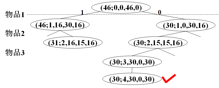
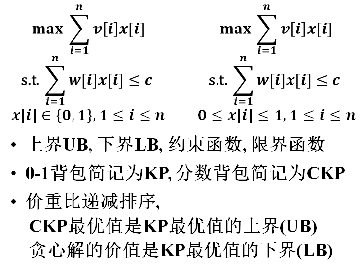
Upper and lower bound design

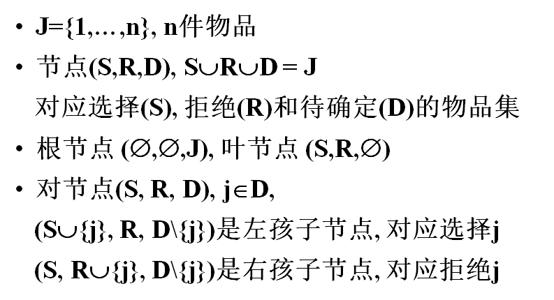
Node design

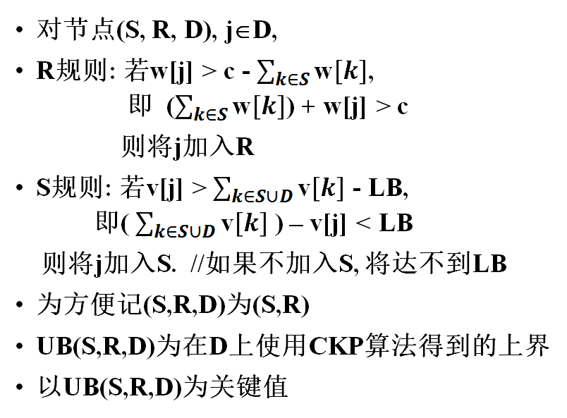
Constraints and limits

give an example