Broadcasting and scientific operation of 03 tensor
1, Broadcast properties of tensors
Tensors have the same broadcast characteristics as Numpy, that is, tensors of different shapes are allowed to operate
1. Tensor calculation of the same shape
In fact, the broadcast property is also used in the operation between tensors with the same shape
t1 = torch.arange(3)
t1
tensor([0, 1, 2])
t1 + t1
tensor([0, 2, 4])
2. Tensor calculation of different shapes
2.1 calculation of scalar and arbitrary shape tensors
Scalars can be calculated with tensors of any shape. The calculation process is to calculate each element of scalars and tensors.
t1 + 1
tensor([1, 2, 3])
t1 + torch.tensor(1)
tensor([1, 2, 3])
t2 = torch.zeros((3, 4))
t2
tensor([[0., 0., 0., 0.],
        [0., 0., 0., 0.],
        [0., 0., 0., 0.]])
t2 + 1
tensor([[1., 1., 1., 1.],
        [1., 1., 1., 1.],
        [1., 1., 1., 1.]])
2.2 calculation between tensors of the same dimension and different shapes
t2.shape
torch.size([3, 4])
t3 = torch.zeros(3, 4, 5)
t3
tensor([[[0., 0., 0., 0., 0.],
         [0., 0., 0., 0., 0.],
         [0., 0., 0., 0., 0.],
         [0., 0., 0., 0., 0.]],

        [[0., 0., 0., 0., 0.],
         [0., 0., 0., 0., 0.],
         [0., 0., 0., 0., 0.],
         [0., 0., 0., 0., 0.]],

        [[0., 0., 0., 0., 0.],
         [0., 0., 0., 0., 0.],
         [0., 0., 0., 0., 0.],
         [0., 0., 0., 0., 0.]]])
t3.shape
torch.Size([3, 4, 5])
t2
tensor([[0., 0., 0., 0.],
        [0., 0., 0., 0.],
        [0., 0., 0., 0.]])
t2.shape
torch.Size([3, 4])
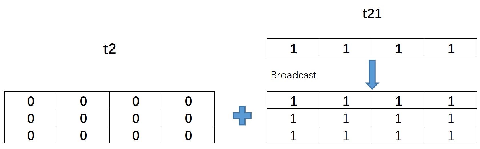
t21 = torch.ones(1, 4)
t21
tensor([[1., 1., 1., 1.]])
The shape of t21 is (1, 4), which is different from the shape of t2 (3, 4) in the first component, but the value of t21 on this component is 1, so it can be broadcast or calculated
t21 + t2
tensor([[1., 1., 1., 1.],
        [1., 1., 1., 1.],
        [1., 1., 1., 1.]])
The broadcast calculation process of t21 and t2 is shown in the following figure:
t22 = torch.ones(3, 1)
t22
tensor([[1.],
        [1.],
        [1.]])
t2
tensor([[0., 0., 0., 0.],
        [0., 0., 0., 0.],
        [0., 0., 0., 0.]])
t2.shape
torch.Size([3, 4])
t22 + t2              # The tensor with shape (3,1) and the tensor with shape (3,4) are added to broadcast
tensor([[1., 1., 1., 1.],
        [1., 1., 1., 1.],
        [1., 1., 1., 1.]])
The actual calculation process of t2 and t22 is as follows: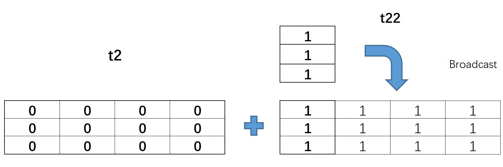
t23 = torch.ones(2, 4)
t23.shape
torch.Size([2, 4])
t2.shape
torch.Size([3, 4])
Note: at this time, the first component dimension of the shape of t2 and t23 is different, but both values are not 1, so they cannot be broadcast
t2 + t23
---------------------------------------------------------------------------

RuntimeError                              Traceback (most recent call last)

<ipython-input-61-994547ec6516> in <module>
----> 1 t2 + t23


RuntimeError: The size of tensor a (3) must match the size of tensor b (2) at non-singleton dimension 0
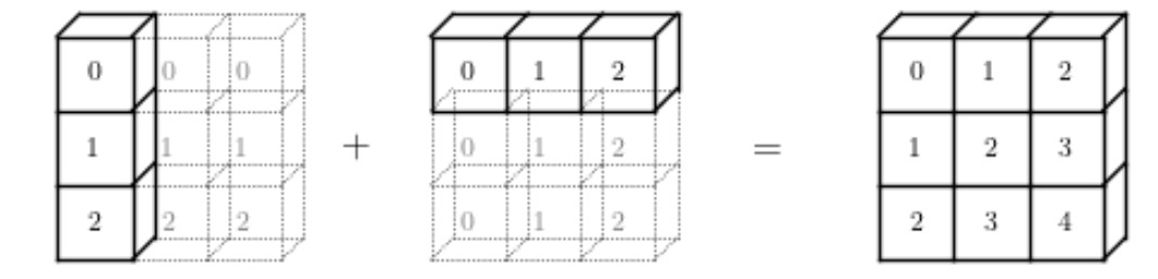
t24 = torch.arange(3).reshape(3, 1)
t24
tensor([[0],
        [1],
        [2]])
t25 = torch.arange(3).reshape(1, 3)
t25
tensor([[0, 1, 2]])
At this time, the shape of t24 is (3,1) and the shape of t25 is (1,3). The two shapes are different in two parts, but there is a case of 1, so they can also be broadcast
t24 + t25
tensor([[0, 1, 2],
        [1, 2, 3],
        [2, 3, 4]])
The calculation process is as follows:
Broadcasting of three-dimensional tensors
t3 = torch.zeros(3, 4, 5)
t3
tensor([[[0., 0., 0., 0., 0.],
         [0., 0., 0., 0., 0.],
         [0., 0., 0., 0., 0.],
         [0., 0., 0., 0., 0.]],

        [[0., 0., 0., 0., 0.],
         [0., 0., 0., 0., 0.],
         [0., 0., 0., 0., 0.],
         [0., 0., 0., 0., 0.]],

        [[0., 0., 0., 0., 0.],
         [0., 0., 0., 0., 0.],
         [0., 0., 0., 0., 0.],
         [0., 0., 0., 0., 0.]]])
t31 = torch.ones(3, 4, 1)
t31
tensor([[[1.],
         [1.],
         [1.],
         [1.]],

       [[1.],
        [1.],
        [1.],
        [1.]],

       [[1.],
        [1.],
        [1.],
        [1.]]])
t3 + t31
tensor([[[1., 1., 1., 1., 1.],
         [1., 1., 1., 1., 1.],
         [1., 1., 1., 1., 1.],
         [1., 1., 1., 1., 1.]],

        [[1., 1., 1., 1., 1.],
         [1., 1., 1., 1., 1.],
         [1., 1., 1., 1., 1.],
         [1., 1., 1., 1., 1.]],

        [[1., 1., 1., 1., 1.],
         [1., 1., 1., 1., 1.],
         [1., 1., 1., 1., 1.],
         [1., 1., 1., 1., 1.]]])
t32 = torch.ones(3, 1, 5)
t32
tensor([[[1., 1., 1., 1., 1.]],

        [[1., 1., 1., 1., 1.]],

       	[[1., 1., 1., 1., 1.]]])
t32 + t3
tensor([[[1., 1., 1., 1., 1.],
         [1., 1., 1., 1., 1.],
         [1., 1., 1., 1., 1.],
         [1., 1., 1., 1., 1.]],

        [[1., 1., 1., 1., 1.],
         [1., 1., 1., 1., 1.],
         [1., 1., 1., 1., 1.],
         [1., 1., 1., 1., 1.]],

        [[1., 1., 1., 1., 1.],
         [1., 1., 1., 1., 1.],
         [1., 1., 1., 1., 1.],
         [1., 1., 1., 1., 1.]]])
If there are two different components in the shape of two tensors, as long as one of the different components is still 1, it can still be broadcast
t3.shape
torch.Size([3, 4, 5])
t33 = torch.ones(1, 1, 5)
t33
tensor([[[1., 1., 1., 1., 1.]]])
t3 + t33
tensor([[[1., 1., 1., 1., 1.],
             [1., 1., 1., 1., 1.],
             [1., 1., 1., 1., 1.],
             [1., 1., 1., 1., 1.]],

            [[1., 1., 1., 1., 1.],
             [1., 1., 1., 1., 1.],
             [1., 1., 1., 1., 1.],
             [1., 1., 1., 1., 1.]],

            [[1., 1., 1., 1., 1.],
             [1., 1., 1., 1., 1.],
             [1., 1., 1., 1., 1.],
             [1., 1., 1., 1., 1.]]])
The calculation process of T3 and t33 is as follows

2.3 broadcast in tensor calculation of different dimensions
# Transformation of two-dimensional tensor into three-dimensional tensor
t2 = torch.arange(4).reshape(2, 2)
t2
tensor([[0, 1],
        [2, 3]])
# Convert to three-dimensional tensor
t2.reshape(1, 2, 2)
tensor([[[0, 1],
         [2, 3]]])
After transformation, it represents a three-dimensional tensor containing only one two-dimensional tensor, and the two-dimensional tensor is t2
# Into a four-dimensional tensor
t2.reshape(1, 1, 2, 2)
tensor([[[[0, 1],
          [2, 3]]]])
After transformation, it represents a four-dimensional tensor containing only one three-dimensional tensor, and the three-dimensional tensor contains only one two-dimensional tensor, and the two-dimensional tensor is t2
t3 = torch.zeros(3, 2, 2)
The calculation process of t3 and t2 is equivalent to two tensors with shapes of (1, 2, 2) and (3, 2, 2)
t3 + t2
tensor([[[0., 1.],
         [2., 3.]],

        [[0., 1.],
         [2., 3.]],

        [[0., 1.],
         [2., 3.]]])
t3 + t2.reshape(1, 2, 2)
tensor([[[0., 1.],
         [2., 3.]],

        [[0., 1.],
         [2., 3.]],

        [[0., 1.],
         [2., 3.]]])
2, Pointwise Ops
Point by point operation mainly includes three parts: basic mathematical operation, numerical adjustment operation and data scientific operation. The related functions are as follows:
| function | describe |
|---|---|
| torch.add(t1,t2 ) | The two tensors t1 and t2 are added element by element, which is equivalent to t1+t2 |
| torch.subtract(t1,t2) | t1 and t2 tensors are subtracted element by element, which is equivalent to t1-t2 |
| torch.multiply(t1,t2) | The two tensors t1 and t2 are multiplied element by element, which is equivalent to t1*t2 |
| torch.divide(t1,t2) | t1 and t2 tensors are divided element by element, which is equivalent to t1/t2 |
t1 = torch.tensor([1, 2])
t1
tensor([1, 2])
t2 = torch.tensor([3, 4])
t2
tensor([3, 4])
torch.add(t1, t2)
tensor([4, 6])
t1 + t2
tensor([4, 6])
Tensor numeric adjustment functiont1 / t2 tensor([0.3333, 0.5000])
| function | describe |
|---|---|
| torch.abs(t) | Return absolute value |
| torch.ceil(t) | Round up |
| torch.floor(t) | Round down |
| torch.round(t) | Rounding |
| torch.neg(t) | Returns the opposite number |
t = torch.randn(5)
t
tensor([-0.5184, -0.4910, -0.1381, -0.2500, -0.4295])
torch.round(t)
tensor([-1., -0., -0., -0., -0.])
torch.abs(t)
tensor([0.5184, 0.4910, 0.1381, 0.2500, 0.4295])
torch.neg(t)
tensor([0.5184, 0.4910, 0.1381, 0.2500, 0.4295])
**Note: * * although this type of function is a numeric adjustment function, it will not adjust the original object, but output a new result.
t # t itself has not changed
tensor([-0.5184, -0.4910, -0.1381, -0.2500, -0.4295])
If you want to modify the original object itself, you can consider using the method_ () to modify the object itself. At this time, the method is the above function with the same name.
t.abs_()
tensor([0.5184, 0.4910, 0.1381, 0.2500, 0.4295])
t
tensor([0.5184, 0.4910, 0.1381, 0.2500, 0.4295])
t.neg_()
tensor([-0.5184, -0.4910, -0.1381, -0.2500, -0.4295])
t
tensor([-0.5184, -0.4910, -0.1381, -0.2500, -0.4295])
In addition to the corresponding homonymous methods for the above numerical adjustment functions, many scientific calculations have homonymous methods.
t.exp_()
tensor([0.5955, 0.6120, 0.8710, 0.7788, 0.6508])
Tensor commonly used scientific computingt tensor([0.5955, 0.6120, 0.8710, 0.7788, 0.6508])
| Mathematical operation function | mathematical formula | describe |
|---|---|---|
| exponentiation | ||
| torch.exp(t) | $ y_{i} = e^{x_{i}} $ | Returns a tensor with e as the base and the element in t as the power |
| torch.expm1(t) | $ y_{i} = e^{x_{i}} $ - 1 | Calculate exp (x) - 1 for all elements in the tensor |
| torch.exp2(t) | $ y_{i} = 2^{x_{i}} $ | Calculate the t-Power of 2 element by element. |
| torch.pow(t,n) | $\text{out}_i = x_i ^ \text{exponent} $ | Returns the nth power of t |
| torch.sqrt(t) | $ \text{out}{i} = \sqrt{\text{input}{i}} $ | Returns the square root of t |
| torch.square(t) | $ \text{out}_i = x_i ^ \text{2} $ | Returns the square of the input element. |
| Logarithmic operation | ||
| torch.log10(t) | $ y_{i} = \log_{10} (x_{i}) $ | Returns the logarithm of t based on 10 |
| torch.log(t) | $ y_{i} = \log_{e} (x_{i}) $ | Returns the logarithm of t based on e |
| torch.log2(t) | $ y_{i} = \log_{2} (x_{i}) $ | Returns the logarithm of t based on 2 |
| torch.log1p(t) | $ y_i = \log_{e} (x_i $ + 1) | Returns an input array plus natural logarithms. |
| Trigonometric function operation | ||
| torch.sin(t) | Triangular sine. | |
| torch.cos(t) | Element cosine. | |
| torch.tan(t) | Calculates tangents on an element by element basis. |
- Most scientific calculations of tensor can only act on tensor objects
# Calculate the power of 2
torch.pow(2, 2)
---------------------------------------------------------------------------

TypeError                                 Traceback (most recent call last)

<ipython-input-124-b05e9bca6d33> in <module>
----> 1 torch.pow(2, 2)


TypeError: pow() received an invalid combination of arguments - got (int, int), but expected one of:
 * (Tensor input, Tensor exponent, *, Tensor out)
 * (Number self, Tensor exponent, *, Tensor out)
 * (Tensor input, Number exponent, *, Tensor out)
torch.pow(torch.tensor(2), 2)
tensor(4)
Note: compared with Python native data type, tensor is a more special kind of object. For example, tensor can be specified to run on CPU or GPU. Therefore, many tensor scientific calculation functions do not allow tensor to be mixed with Python native numerical objects.
- Most scientific operations of tensor are static
The so-called staticality means that there are clear requirements for the input tensor type. For example, some functions can only input floating-point tensors, not integer tensors.
t = torch.arange(1, 4)
t.dtype
torch.int64
torch.exp(t)
---------------------------------------------------------------------------

RuntimeError                              Traceback (most recent call last)

<ipython-input-103-ad3d5759497c> in <module>
----> 1 torch.exp(t)


RuntimeError: exp_vml_cpu not implemented for 'Long'
It should be noted that although Python is a dynamically compiled programming language, in PyTorch, because GPU calculation is involved, the element type will not be adjusted during actual function calculation. Most of the scientific operations here require the object type to be floating-point, and type conversion is required in advance.
t1 = t.float()
t1
tensor([1., 2., 3.])
torch.exp(t1)
tensor([ 2.7183,  7.3891, 20.0855])
torch.expm1(t1)
tensor([ 1.7183,  6.3891, 19.0855])
torch.exp2(t1)
tensor([2., 4., 8.])
torch.pow(t, 2)
tensor([1, 4, 9])
Pay attention to distinguish the t power of 2 from the 2 power of T
torch.square(t)
tensor([1, 4, 9])
torch.sqrt(t1)
tensor([1.0000, 1.4142, 1.7321])
torch.pow(t1, 0.5)
tensor([1.0000, 1.4142, 1.7321])
The open radical is equal to 0.5 power
torch.log10(t1)
tensor([0.0000, 0.3010, 0.4771])
torch.log(t1)
tensor([0.0000, 0.6931, 1.0986])
torch.log2(t1)
tensor([0.0000, 1.0000, 1.5850])
torch.exp(torch.log(t1))
tensor([1., 2., 3.])
torch.exp2(torch.log2(t1))
tensor([1., 2., 3.])
a = torch.tensor(-1).float()
a
tensor(-1.)
torch.exp2(torch.log2(a))
tensor(nan)
- Sort operation: sort
In PyTorch, the sort sort function will return both the sort result and the arrangement of the corresponding index values.
t = torch.tensor([1.0, 3.0, 2.0])
t
tensor([1., 3., 2.])
# Ascending arrangement
torch.sort(t)
torch.return_types.sort(
    values=tensor([1., 2., 3.]),
    indices=tensor([0, 2, 1]))
# Descending order
torch.sort(t, descending=True)
torch.return_types.sort(
    values=tensor([3., 2., 1.]),
    indices=tensor([1, 2, 0]))
3, Protocol operation
Conventional operation refers to a function that summarizes a tensor and finally obtains a specific summary value. Such functions mainly include many statistical analysis functions in the field of data science, such as mean, extreme value, variance, median function and so on.
Tensor statistical analysis function| function | describe |
|---|---|
| torch.mean(t) | Return tensor mean |
| torch.var(t) | Return tensor variance |
| torch.std(t) | Return tensor standard deviation |
| torch.var_mean(t) | Returns the tensor variance and mean |
| torch.std_mean(t) | Returns the tensor standard deviation and mean |
| torch.max(t) | Returns the maximum tensor |
| torch.argmax(t) | Returns the tensor maximum index |
| torch.min(t) | Returns the minimum value of the tensor |
| torch.argmin(t) | Returns the tensor minimum index |
| torch.median(t) | Returns the median tensor |
| torch.sum(t) | Returns the tensor summation result |
| torch.logsumexp(t) | Returns the summation result of tensor elements, which is applicable to the case of small amount of data |
| torch.prod(t) | Returns the tensor multiplication result |
| torch.dist(t1, t2) | Different paradigms can be used to calculate the Min distance of two tensors |
| torch.topk(t) | Returns the indicator corresponding to the largest k values in t |
# Generate floating point tensor
t = torch.arange(10).float()
t
tensor([0., 1., 2., 3., 4., 5., 6., 7., 8., 9.])
# Calculated mean
torch.mean(t)
tensor(4.5000)
# Calculate standard deviation and mean
torch.std_mean(t)
(tensor(3.0277), tensor(4.5000))
# Calculate maximum
torch.max(t)
tensor(9.)
# Returns the index of the maximum value
torch.argmax(t)
tensor(9)
# Calculate median
torch.median(t)
tensor(4.)
# Sum
torch.sum(t)
tensor(45.)
# quadrature
torch.prod(t)
tensor(0.)
torch.prod(torch.tensor([1, 2, 3]))
tensor(6)
t1 = torch.tensor([1.0, 2])
t1
tensor([1., 2.])
t2 = torch.tensor([3.0, 4])
t2
tensor([3., 4.])
t
tensor([0., 1., 2., 3., 4., 5., 6., 7., 8., 9.])
- dist calculated distance
dist function can calculate min distance (Minkowski distance). By entering different p values, you can calculate various types of distances, such as European distance, street distance, etc. Minkowski distance formula is as follows:
$ D(x,y) = (\sum^{n}_{u=1}|x_u-y_u|^{p})^{1/p}$When p is 2, the Euclidean distance is calculated
torch.dist(t1, t2, 2)
tensor(2.8284)
torch.sqrt(torch.tensor(8.0))
tensor(2.8284)
When p is 1, the street distance is calculated
torch.dist(t1, t2, 1)
tensor(4.)
Several distances commonly used in machine learning are shown in the following figure: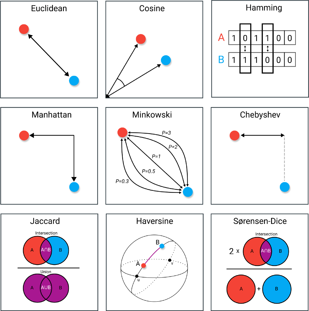
Reference link: https://towardsdatascience.com/9-distance-measures-in-data-science-918109d069fa
- Dimension of specification operation
Since the specification operation is a sequence that returns a result, if it is for a high-dimensional tensor, a dimension can be specified for calculation.
# Create a 3 * 3 two-dimensional tensor
t2 = torch.arange(12).float().reshape(3, 4)
t2
tensor([[ 0.,  1.,  2.,  3.],
            [ 4.,  5.,  6.,  7.],
            [ 8.,  9., 10., 11.]])
t2.shape
torch.Size([3, 4])
# Sum by the first dimension (three at a time) and by column
torch.sum(t2, dim = 0)
tensor([12., 15., 18., 21.])
# Sum according to the second dimension (four at a time) and sum according to rows
torch.sum(t2, dim = 1)
tensor([ 6., 22., 38.])
# Create a 2 * 3 * 4 three-dimensional tensor
t3 = torch.arange(24).float().reshape(2, 3, 4)
t3
tensor([[[ 0.,  1.,  2.,  3.],
         [ 4.,  5.,  6.,  7.],
         [ 8.,  9., 10., 11.]],

        [[12., 13., 14., 15.],
         [16., 17., 18., 19.],
         [20., 21., 22., 23.]]])
t3.shape
torch.Size([2, 3, 4])
torch.sum(t3, dim = 0)
tensor([[12., 14., 16., 18.],
        [20., 22., 24., 26.],
        [28., 30., 32., 34.]])
torch.sum(t3, dim = 1)
tensor([[12., 15., 18., 21.],
        [48., 51., 54., 57.]])
torch.sum(t3, dim = 2)
tensor([[ 6., 22., 38.],
        [54., 70., 86.]])
Note: the dim parameter corresponds to the returned result of shape one by one.
- Ordering of two-dimensional tensors
Similar to the above process, in the sorting process, the two-dimensional tensor can also be sorted by row or column
t22 = torch.randn(3, 4)             # Creating a two-dimensional random number tensor
t22
tensor([[ 0.0274, -1.1111, -0.0721,  0.0524],
        [-0.1148, -1.5132, -0.0838,  0.4069],
        [-0.9713, -0.9050, -0.4375, -0.6726]])
# By default, it is sorted in ascending order by row
torch.sort(t22)
torch.return_types.sort(
    values=tensor([[-1.1111, -0.0721,  0.0274,  0.0524],
            [-1.5132, -0.1148, -0.0838,  0.4069],
            [-0.9713, -0.9050, -0.6726, -0.4375]]),
    indices=tensor([[1, 2, 0, 3],
            [1, 0, 2, 3],
            [0, 1, 3, 2]]))
# Modify the dim and descending parameters to sort by column in descending order
torch.sort(t22, dim = 1, descending=True)
torch.return_types.sort(
    values=tensor([[ 0.0524,  0.0274, -0.0721, -1.1111],
            [ 0.4069, -0.0838, -0.1148, -1.5132],
            [-0.4375, -0.6726, -0.9050, -0.9713]]),
    indices=tensor([[3, 0, 2, 1],
            [3, 2, 0, 1],
            [2, 3, 1, 0]]))
4, Comparison operation
comparison operation is a relatively simple operation type, which is similar to Python's native Boolean operation. It is often used for logical operation between different tensors, and finally returns the logical operation result (logical type tensor). The basic comparison operation functions are as follows:
Tensor comparison function| function | describe |
|---|---|
| torch.eq(t1, t2) | Compare whether the elements t1 and t2 are equal and equivalent== |
| torch.equal(t1, t2) | Judge whether the two tensors are the same tensor |
| torch.gt(t1, t2) | Compare whether each element of t1 is greater than each element of t2, equivalent > |
| torch.lt(t1, t2) | Compare whether each element of t1 is less than each element of t2, equivalent< |
| torch.ge(t1, t2) | Compare whether each element of t1 is greater than or equal to each element of t2, equivalent >= |
| torch.le(t1, t2) | Compare whether each element of t1 is less than or equal to each element of t2, equivalent<= |
| torch.ne(t1, t2) | Compare whether t1 and t2 elements are different and equivalent= |
t1 = torch.tensor([1.0, 3, 4])
t2 = torch.tensor([1.0, 2, 5])
t1 == t2
tensor([ True, False, False])
torch.equal(t1, t2)          # Judge whether t1 and t2 are the same tensors
False
torch.eq(t1, t2)
tensor([ True, False, False])
t1 > t2
tensor([False,  True, False])
t1 >= t2
tensor([ True,  True, False])