1 company introduction

Morphl is a foreign company providing AI solutions (PS: this company has a nice web UI ~):
website: https://morphl.io/products/morphl-cloud.html

MorphL Community Edition
MorphL Community Edition uses big data and machine learning to predict user behavior in digital products and services. Its goal is to improve KPI (click through rate, conversion rate, etc.) through personalization. The main models include:

• Model 1: crowd shopping stage - circle selection of high potential buyers;
  Pinpoint users who are more likely to join the shopping cart, check out or complete the transaction.
• Model 2: shopping loss model cart environment - circle selection of people who are easy to lose;
  Pinpoint users who are more likely to give up their shopping cart in the current or next round.
• Model 3: Customers LTV - lifecycle model
  Reduce customer churn and turn them into loyal customers by focusing on users with low or medium customer lifetime value.
• Personalized recommendation model
• Associated product model
• High frequency purchase model
• Search intention
• Population classification
• Loss warning
  

2 budget allocation

In the morphl theoretical system, budget allocation includes two steps:

• Calculate the functional relationship between budget - > revenue
• Calculate the budget allocation optimization model for each activity

Step 1 budget / revenue forecast function

f(Cost) = f(Cost(t) | Cost(t-1), Revenue(t-1), ... Cost(t0), Revenue(t0)) = Revenue function

Forecast based on historical budget / revenue data

Step 2 budget optimization
Once you have the budget / revenue forecast function for each activity, you can start to solve the budget optimization. There are three cases:

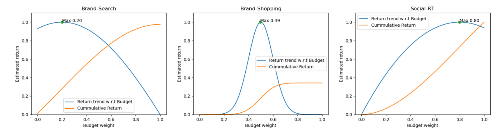
The yellow line is the cumulative line of budget / input amount;
The blue line is the relationship between the budget and the returning sum

The vertex of the curve is the best buffer range, which can help with budge t allocation

3. Interpretation of relevant cases

3.1 relevant data style

github address: Morphl-AI/Ecommerce-Marketing-Spend-Optimization

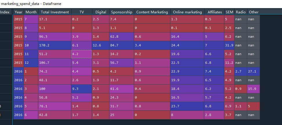
Look at the two data source formats released by github:

• Market spending data, including year, total investment, TV/Digital and other channel revenue
• Channel conversion data, advertising ID, FB activity ID, age, gender, exposure, click, cost, conversion, etc
  

Several cases introduce their common methods:

3.2 2. Budget optimization - basic statistical model

Here are actually several very simple methods

• Income ~ input, ROI calculated by direct division
• Income exposure and exposure input are also direct division conversion

3.3 4. Budget allocation - pseudo-revenue - first-revenue assumption - regressions

• The regression model is used to calculate Revenue~cost
• Two methods are illustrated, Revenue ~ cost two variable regression; Covariates such as rev ~ cost + click
  Here is a bucket index concept, which is not particularly understood. It is speculated that it is a reasonable activity interval, similar to session

Let a bucket be: C o s t B = [ 0 , 0 , 50 , 20 , 0 , 15 ] Cost_B=[0, 0, 50, 20, 0, 15] CostB​=[0,0,50,20,0,15], R e v e n u e B = [ 30 , 100 ] Revenue_B=[30, 100] RevenueB​=[30,100].
This means that the first revenue (30) was generated by the first two costs alone,
so we merged the next bucket as well.
We'll sum them, getting C Σ B = 85 C_{\Sigma B}=85 CΣB​=85 and R Σ B = 130 R_{\Sigma B}=130 RΣB​=130. Then, the bucket constant is: α B = 130 / 85 = 1.529 \alpha_B=130/85=1.529 αB​=130/85=1.529.
Then, our pseudo-revenues will be: P s e u d o − R e v e n u e B = [ 0 ∗ α B , 0 ∗ α B , 50 ∗ α B , 20 ∗ α B , 0 ∗ α B , 15 ∗ α B ] = [ 0 , 0 , 76.45 , 30.58 , 0 , 22.935 ] Pseudo-Revenue_{B} = [0*\alpha_B, 0*\alpha_B, 50*\alpha_B, 20*\alpha_B, 0*\alpha_B, 15*\alpha_B] = [0, 0, 76.45, 30.58, 0, 22.935] Pseudo−RevenueB​=[0∗αB​,0∗αB​,50∗αB​,20∗αB​,0∗αB​,15∗αB​]=[0,0,76.45,30.58,0,22.935].

With the help of the above examples, I guess,

• Why not one-to-one correspondence: [ 0 , 0 , 50 , 20 , 0 , 15 ] − > [ r 1 , r 2 , r 3 , r 4 , r 5 ] [0,0,50,20,0,15] -> [r1,r2,r3,r4,r5] [0,0,50,20,0,15]−>[r1,r2,r3,r4,r5]
  Because the input and statistical income are not synchronized, it will take some time to count after the input.
• How to correspond one by one?
  Some data interpolation strategies can be adopted, such as calculating a total bucket constant

3.4 5. Budget allocation - pseudo-revenue - one-week assumption - regressions

The fourth case may be intermittent activities, and the fifth case may be a long-term case,
Therefore, the bucket interval here is a fixed one week, which is used for calculation.

4 code test

github address: Morphl-AI/Ecommerce-Marketing-Spend-Optimization

Look at the two data source formats released by github:

• Market spending data, including year, total investment, TV/Digital and other channel revenue
• Channel conversion data, advertising ID, FB activity ID, age, gender, exposure, click, cost, conversion, etc

4.1 simple coefficient first-order revenue forecast

Corresponding to jupyter - 2 Budget optimization - basic statistical model

Direct = > R e v / C o s t Rev / Cost Rev/Cost

import pandas as pd

'''
Model 1: directly calculate the total ROI
Directly modeling f(Cost) = Revenue
'''
class StatisticalModel:
    def __init__(self):
        # This model has just a single parameter, computed as the count between targets and inputs
        self.param = np.nan
        
    def fit(self, x, t):
        assert self.param != self.param
        self.param = t.sum() / x.sum()  # Core, a very simple ROI is calculated as a coefficient
    
    def predict(self, x):
        assert self.param == self.param
        return x * self.param
    
def errorL1(y, t):
    return np.abs(y - t).mean()

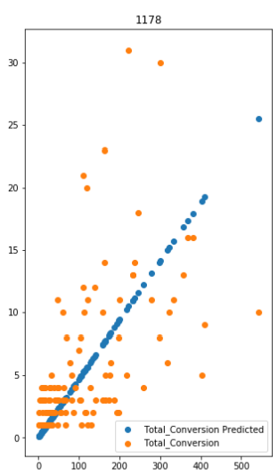
def plot(model, valData, xKey, tKey):
    validCampaigns = list(valData.keys())
    ax = plt.subplots(len(validCampaigns), figsize=(5, 30))[1]
    for i, k in enumerate(validCampaigns):
        x = valData[k][xKey]
        t = valData[k][tKey]
        y = model[k].predict(x)
        ax[i].scatter(x, y, label="%s Predicted" % (tKey))
        ax[i].scatter(x, t)
        ax[i].set_title(k)
        ax[i].legend()

# Data read in

conversion_data = pd.read_csv('Datasets/conversion_data.csv')
# marketing_spend_data = pd.read_csv('Datasets/marketing_spend_data.csv')


model_cost_revenue = {}
predictions_cost_revenue = {}
errors_cost_revenue = {}
displayDf = pd.DataFrame()
res_cost_revenue = []

campaigns = set(conversion_data['xyz_campaign_id'])
# from sklearn.model_selection import train_test_split
# X_train,X_test,y_train,y_test = train_test_split(iris.data,iris.target,test_size=0.3,random_state=0)
trainData = {}
valData = {}
for k in campaigns:
    data = conversion_data[conversion_data['xyz_campaign_id'] == k]
    num = int(len(data)*0.8)
    trainData[k] = data[:num]
    valData[k] = data[num:]

# Cost_col = 'Cost'
# Revenue_col = 'Revenue'
Cost_col = 'Spent'  # investment
Revenue_col = 'Total_Conversion' # produce

for k in campaigns:
    model_cost_revenue[k] = StatisticalModel()
    model_cost_revenue[k].fit(trainData[k][Cost_col], trainData[k][Revenue_col])
    predictions_cost_revenue[k] = model_cost_revenue[k].predict(valData[k][Cost_col])
    errors_cost_revenue[k] = errorL1(predictions_cost_revenue[k], valData[k][Revenue_col])
    res_cost_revenue.append([k, trainData[k][Cost_col].sum(), trainData[k][Revenue_col].sum(), \
                model_cost_revenue[k].param, errors_cost_revenue[k]])


displayDf = pd.DataFrame(res_cost_revenue, columns=["Campaign", Cost_col, Revenue_col, "Fit", "Error (L1)"])
display(displayDf)
print("Mean error:", displayDf["Error (L1)"].mean())

plot(model_cost_revenue, valData, Cost_col, Revenue_col)

Just an example,

4.2 model II: consider exposure

Similar: cost - > exposure - > revenue

Cost x Revenue ~= Cost x Sessions + Sessions x Revenue

exposure = a1 * cost
 income = a2 * exposure

It is divided into two steps, and the main interception is also 2 Budget optimization - basic statistical model

# Set a session randomly
session_col = 'Impressions' # exposure
Cost_col = 'Spent'  # investment
Revenue_col = 'Total_Conversion' # produce

# Step 1: exposure = a1 * cost
model_cost_sessions = {}
predictions_cost_sessions = {}
errors_cost_sessions = {}
displayDf = pd.DataFrame()
res_cost_sessions = []
for k in campaigns:
    model_cost_sessions[k] = StatisticalModel()
    model_cost_sessions[k].fit(trainData[k][Cost_col], trainData[k][session_col])
    predictions_cost_sessions[k] = model_cost_sessions[k].predict(valData[k][Cost_col])
    errors_cost_sessions[k] = errorL1(predictions_cost_sessions[k], valData[k][session_col])
    res_cost_sessions.append([k, trainData[k][Cost_col].sum(), trainData[k][session_col].sum(), \
                model_cost_sessions[k].param, errors_cost_sessions[k]])

displayDf = pd.DataFrame(res_cost_sessions, columns=["Campaign", Cost_col, session_col, "Fit", "Error (L1)"])
display(displayDf)
print("Mean error:", displayDf["Error (L1)"].mean())

plot(model_cost_sessions, valData, Cost_col, session_col)

# Step 2: revenue = a2 * exposure
model_sessions_revenue = {}
predictions_sessions_revenue = {}
errors_sessions_revenue = {}
displayDf = pd.DataFrame()
res_sessions_revenue = []
for k in campaigns:
    model_sessions_revenue[k] = StatisticalModel()
    model_sessions_revenue[k].fit(trainData[k][session_col], trainData[k][Revenue_col])
    predictions_sessions_revenue[k] = model_sessions_revenue[k].predict(valData[k][session_col])
    errors_sessions_revenue[k] = errorL1(predictions_sessions_revenue[k], valData[k][Revenue_col])
    res_sessions_revenue.append([k, trainData[k][session_col].sum(), trainData[k][Revenue_col].sum(), \
                model_sessions_revenue[k].param, errors_sessions_revenue[k]])

displayDf = pd.DataFrame(res_sessions_revenue, columns=["Campaign", session_col, Revenue_col, "Fit", "Error (L1)"])
display(displayDf)
print("Mean error:", displayDf["Error (L1)"].mean())

plot(model_sessions_revenue, valData, session_col, Revenue_col)

# Step 3: Merge
displayDf = pd.DataFrame()
errors_cost_revenue = {}
res_cost_revenue_combined = []

class TwoModel(object):
    def __init__(self, modelA, modelB):
        self.modelA = modelA
        self.modelB = modelB
    
    def predict(self, x):
        return self.modelA.predict(self.modelB.predict(x))
models_cost_revenue = {k : TwoModel(model_cost_sessions[k], model_sessions_revenue[k]) for k in valData}

for k in campaigns:
    predictions_cost_revenue[k] = models_cost_revenue[k].predict(valData[k][Cost_col])
    errors_cost_revenue[k] = errorL1(predictions_cost_revenue[k], valData[k][Revenue_col])
    res_cost_revenue_combined.append([k, errors_cost_revenue[k]])

displayDf = pd.DataFrame(res_cost_revenue_combined, columns=["Campaign", "Error (L1)"])
display(displayDf)
print("Mean error:", displayDf["Error (L1)"].mean())


plot(models_cost_revenue, valData, Cost_col, Revenue_col)