TensorFlow is a python-based framework for machine learning. After learning the course content of Logical Regression in Coursera, I want to re-implement the content implemented in MATLAB with TensorFlow as a knocking brick for learning Python and framework.

Target readers

Know what logistic regression is, know a little Python, have heard of TensorFlow

data set

From Andrew's machine learning course in Coursera, ex2data1.txt, the student's two test scores are used to determine whether the student will be admitted or not.

Environmental Science

Python 2.7 - 3.x

pandas, matplotlib, numpy

Install TensorFlow

Installation of TensorFlow framework on your computer, installation process is not detailed, CPU version is relatively easier, GPU version needs CUDA support, you can see the situation of installation.

start

Create a folder (such as tensorflow), create a Python file main.py in the folder, and place the data set file under this folder:

Data form:

The first two columns are the results of two examinations (x1, x2), the last one is whether or not to be admitted (y), one is to be admitted, and the other is 0.

In the main.py source file, we first introduce the required packages:

import pandas as pd                # Used to read data files
import tensorflow as tf
import matplotlib.pyplot as plt    # Used for drawing
import numpy as np                 # For subsequent calculation

pandas is a data processing related package that can read data sets and perform various other operations; matplotlib can be used to map and display our data.

Then we read the data set file into the program for later training:

# Read data files
df = pd.read_csv("ex2data1.txt", header=None)
train_data = df.values

The pandas function read_csv can read the data in the CSV (comma-separated values) file into the DF variable and convert the DataFrame into a two-dimensional array through df.values:

After we have the data, we need to put the features (x1, x2) and labels (y) into two variables respectively in order to substitute the formulas in the training:

# Separation of features and labels and acquisition of data dimension
train_X = train_data[:, :-1]
train_y = train_data[:, -1:]
feature_num = len(train_X[0])
sample_num = len(train_X)
print("Size of train_X: {}x{}".format(sample_num, feature_num))
print("Size of train_y: {}x{}".format(len(train_y), len(train_y[0])))

As you can see, there are 100 samples in our data set, and the number of features per sample is 2.

TensorFlow Model Design

In logistic regression, we use the prediction function (Hypothesis) as follows:

$$
h_θ(x) = sigmoid(XW + b)
$$

Among them, sigmoid is an activation function, which indicates the probability of students being admitted:

$$
P(y = 1 | x, \theta)
$$

The shape of this function, please Baidu

W and b are our next learning goals, W is the weight matrix (Weights), b is the offset (Bias, reflected in the image is also called intercept).

The loss function we use is:

$$
J(θ) = -\frac{1}{m} \left[ \sum_{i=1}^m y^{(i)}\log(h_\theta(x^{(i)})) + (1 - y^{(i)})\log(1 - h_\theta(x^{(i)})) \right]
$$

Since our data set has only two features, we don't need to worry about over-fitting, so we don't need the normalization term in the loss function.

First, we define two variables with TensorFlow to store our training data:

# data set
X = tf.placeholder(tf.float32)
y = tf.placeholder(tf.float32)

Here, X and y are not general variables, but a placeholder (placeholder), which means that the values of these two variables are unspecified, and you don't need to assign the given data to the variables until you start training the model.

Then we define W and b that we want to train.

# Training objectives
W = tf.Variable(tf.zeros([feature_num, 1]))
b = tf.Variable([-.9])

Here their type is Variable, which means that these two variables will change continuously during the training iteration, and ultimately achieve the desired value. As you can see, we set the initial value of W to the 0 vector of feature_num dimension and the initial value of b to -0.9.

Next, we use TensorFlow to express the loss function.

db = tf.matmul(X, tf.reshape(W, [-1, 1])) + b
hyp = tf.sigmoid(db)

cost0 = y * tf.log(hyp)
cost1 = (1 - y) * tf.log(1 - hyp)
cost = (cost0 + cost1) / -sample_num
loss = tf.reduce_sum(cost)

It can be seen that the loss function is expressed in three steps: first, the two parts of the sum are expressed separately, then they are added and combined with the external constant m. Finally, the value of the loss function is obtained by summing the vector.

Next, we define the optimization methods used:

optimizer = tf.train.GradientDescentOptimizer(0.001)
train = optimizer.minimize(loss)

Among them, the first step is to select the optimizer, where we choose the gradient descent method; the second step is to optimize the objective, as the function name implies, our optimization goal is to minimize the value of the loss function.

Note: The learning rate here (0.001) should be as small as possible, otherwise it may occur. log(0) appears in loss calculation Questions.

train

After the above work is done, we can begin to train our model.

In TensorFlow, you first initialize the previously defined Variable:

init = tf.global_variables_initializer()
sess = tf.Session()
sess.run(init)

Here, we see a tf.Session(), which, as its name implies, is the subject of task execution. We defined a bunch of things above, just the execution steps and framework needed by a model to get results. A flow chart is not enough. We need a body to actually run it. That's the role of Session.

------------------------------------------------------------------------------------------------------------------------------

If you're using the TensorFlow GPU version and you want to train the model in high graphics card occupancy situations (such as playing games), you should pay attention to initializing Session. Allocate a fixed amount of display memory for it Otherwise, you may drop out directly at the beginning of the training:

2017-06-27 20:39:21.955486: E c:\tf_jenkins\home\workspace\release-win\m\windows-gpu\py\35\tensorflow\stream_executor\cuda\cuda_blas.cc:365] failed to create cublas handle: CUBLAS_STATUS_ALLOC_FAILED
Traceback (most recent call last):
  File "C:\Users\DYZ\Anaconda3\envs\tensorflow\lib\site-packages\tensorflow\python\client\session.py", line 1139, in _do_call
    return fn(*args)
  File "C:\Users\DYZ\Anaconda3\envs\tensorflow\lib\site-packages\tensorflow\python\client\session.py", line 1121, in _run_fn
    status, run_metadata)
  File "C:\Users\DYZ\Anaconda3\envs\tensorflow\lib\contextlib.py", line 66, in __exit__
    next(self.gen)
  File "C:\Users\DYZ\Anaconda3\envs\tensorflow\lib\site-packages\tensorflow\python\framework\errors_impl.py", line 466, in raise_exception_on_not_ok_status
    pywrap_tensorflow.TF_GetCode(status))
tensorflow.python.framework.errors_impl.InternalError: Blas GEMV launch failed:  m=2, n=100
         [[Node: MatMul = MatMul[T=DT_FLOAT, transpose_a=false, transpose_b=false, _device="/job:localhost/replica:0/task:0/gpu:0"](_arg_Placeholder_0_0/_3, Reshape)]]

At this point you need to create Session in the following way:

gpu_options = tf.GPUOptions(per_process_gpu_memory_fraction=0.333)
sess = tf.Session(config=tf.ConfigProto(gpu_options=gpu_options))

Here 0.333 is your share of total memory.

End Special Tip

The following is to train the model with our data set:

feed_dict = {X: train_X, y: train_y}

for step in range(1000000):
    sess.run(train, {X: train_X, y: train_y})
    if step % 100 == 0:
        print(step, sess.run(W).flatten(), sess.run(b).flatten())

First of all, we need to store the incoming data in a variable, and pass in sess.run() when we train the model; we train 10,000 times, every 100 times.
The current target parameters W, b are output once.

At this point, the training code is complete, and you can use your own python command to run it. If you follow the above code strictly and there are no errors, you should now see that the console has started to output training status continuously:

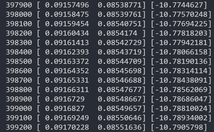
Graphical representation of results

When the training is over, you can get a W, and a b, so that we can visually display the data set and the fitting results through the chart.

In the process of writing, I trained a result with the above code:

We write it directly into the code, that is:

w = [0.12888144, 0.12310864]
b = -15.47322273

Let's first represent the data set on the graph (x1 is the horizontal axis and x2 is the vertical axis):

x1 = train_data[:, 0]
x2 = train_data[:, 1]
y = train_data[:, -1:]

for x1p, x2p, yp in zip(x1, x2, y):
    if yp == 0:
        plt.scatter(x1p, x2p, marker='x', c='r')
    else:
        plt.scatter(x1p, x2p, marker='o', c='g')

Among them, we use red x to represent not being admitted, and green o to represent being admitted.

Secondly, we present the trained decision boundary XW + b = 0 on the chart:

# Get a straight line according to the parameters
x = np.linspace(20, 100, 10)
y = []
for i in x:
    y.append((i * -w[1] - b) / w[0])
    
plt.plot(x, y)
plt.show()

At this point, if your code is correct, run it again and you will get the following results:

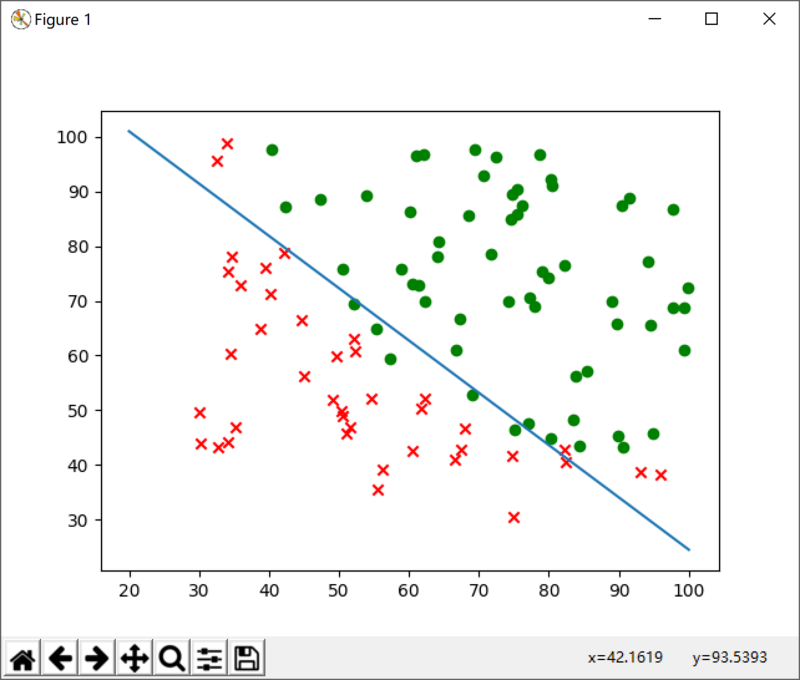
As you can see, we can draw a straight line through the parameters obtained by training, which is very suitable to distinguish two different data samples.

So far, a complete and simple logistic regression model has been implemented. I hope that through this article, you can have a preliminary understanding of the implementation of machine learning model in TensorFlow. I am also in the preliminary study, if there is something wrong welcome in the comment area, in the process of implementing the above code, if you encounter any problems, please open fire at will in the comment area.