 Rimeng Society
AI AI:Keras PyTorch MXNet TensorFlow PaddlePaddle deep learning real combat (irregular update)
4.6 TF common function modules
4.6. 1. Detailed explanation of callback of fit
Callbacks are a set of functions that are applied at a given stage of the training process. Callbacks can be used to obtain views of internal status and model statistics during training. You can pass the callback list (as the keyword parameter callbacks) to the fit() method of the or class. The relevant methods of the callback will then be called at each stage of the training.
- Customized preservation model
- Save events file
4.6.1.1 ModelCheckpoint
from tensorflow.python.keras.callbacks import ModelCheckpoint
- keras.callbacks.ModelCheckpoint(filepath, monitor='val_loss', save_best_only=False, save_weights_only=False, mode='auto', period=1)
- Save the model after every iteration
- filepath: save model string
- If you set weights {epoch:02d}-{val_loss:.2f}. In HDF5 format, the number will be every epoch number, and the loss of validation set will be saved in this location
- If you set weights {epoch:02d}-{val_acc:.2f}. HDF5, will follow val_ ACC value to save the model
- monitor: quantity to monitor. Set to 'Val'_ ACC 'or' Val '_ loss'
- save_best_only: if save_best_only=True, only better results than the last model are retained
- save_weights_only: if True, only the (model.save_weights(filepath)), else the full model is saved (model.save(filepath))
- mode: one of {auto, min, max}. If save_best_only=True for val_acc, to set max, for val_loss to set min
- period: the interval between iteratively saving checkpoints
check = ModelCheckpoint('./ckpt/singlenn_{epoch:02d}-{val_acc:.2f}.h5',
                                monitor='val_acc',
                                save_best_only=True,
                                save_weights_only=True,
                                mode='auto',
                                period=1)

SingleNN.model.fit(self.train, self.train_label, epochs=5, callbacks=[check], validation_data=(x, y))
Note: to use ModelCheckpoint, you must specify the validation set in fit, otherwise an error will be reported.
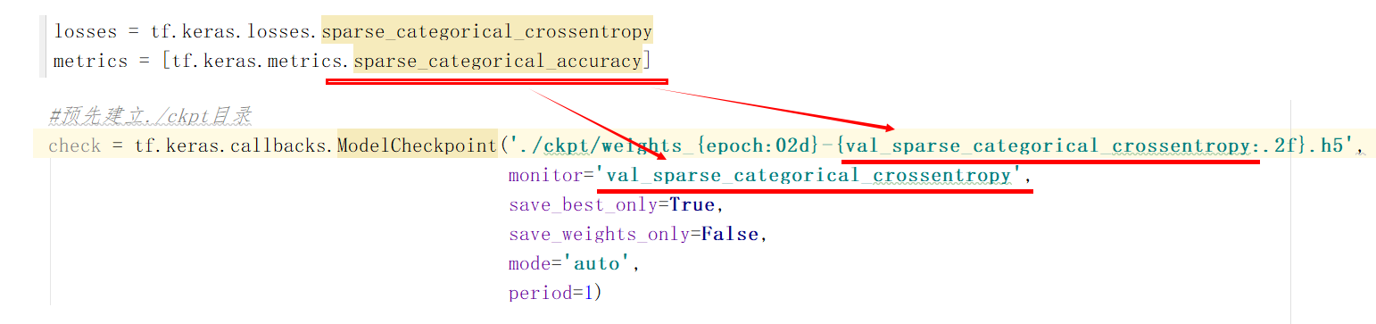
metrics yes sparse_categorical_crossentropy,be ModelCheckpoint The first road strength string information in monitor Required in all parameters val_sparse_categorical_crossentropy
metrics yes acc,be ModelCheckpoint The first road strength string information in monitor Required in all parameters val_acc
metrics yes accuracy,be ModelCheckpoint The first road strength string information in monitor Required in all parameters val_accuracy

4.6.1.2 Tensorboard
- Add Tensorboard to observe the loss, etc
- keras.callbacks.TensorBoard(log_dir='./logs', histogram_freq=0, batch_size=32, write_graph=True, write_grads=False, write_images=False, embeddings_freq=0, embeddings_layer_names=None, embeddings_metadata=None, embeddings_data=None, update_freq='epoch')
- log_dir: directory where event files are saved
- write_graph=True: whether to display the graph structure
- write_images=False: whether to display pictures
- write_grads=True: display gradient histogram_freq , must be greater than 0
# Add tensoboard observation
 tensorboard = keras.callbacks.TensorBoard(log_dir='./graph', histogram_freq=1,
                                                  write_graph=True, write_images=True)

SingleNN.model.fit(self.train, self.train_label, epochs=5, callbacks=[tensorboard])
- Open the terminal to view:
# Specify the directory where the file exists and open the following command
tensorboard --logdir="./"
4.6.2 tf.data: data set construction and preprocessing
- Problem introduction:
Most of the time, we want to use our own data set to train the model. However, in the face of a pile of raw data files with different formats, the process of preprocessing and reading them into the program is often very cumbersome, even more energy-consuming than the design of the model. For example, in order to read in a batch of image files, We may need various image processing packages tangled with python For example, the first mock exam of pillow is to design Batch, and it may not be satisfactory in running. For this reason, TensorFlow provides tf.data module, which includes a flexible data set to build API, which can help us to build data input pipeline quickly and efficiently, especially for large data scenarios.
4.6. 2.1 establishment of dataset object
- tf. The core of data is TF data. Dataset class, which provides high-level encapsulation of data sets.
- tf. data. A dataset consists of a series of iteratively accessible elements, each of which contains one or more tensors. For example, for a dataset composed of images, each element can be a long shape × wide × The picture tensor of the number of channels can also be a Tuple composed of picture tensor and picture label tensor.
1,tf.data.Dataset.from_tensor_slices()
The most basic establishment TF data. The method of dataset is to use TF data. Dataset. from_ tensor_ Slices (), which is applicable to the case where the amount of data is small (it can be loaded into memory as a whole).
import tensorflow as tf
import numpy as np

X = tf.constant([2015, 2016, 2017, 2018, 2019])
Y = tf.constant([12000, 14000, 15000, 16500, 17500])

# You can also use NumPy array with the same effect
# X = np.array([2015, 2016, 2017, 2018, 2019])
# Y = np.array([12000, 14000, 15000, 16500, 17500])

dataset = tf.data.Dataset.from_tensor_slices((X, Y))

for x, y in dataset:
    print(x.numpy(), y.numpy())
output
2013 12000
2014 14000
2015 15000
2016 16500
2017 17500
Similarly, we can load the MNIST dataset in the previous chapter:
import matplotlib.pyplot as plt

(train_data, train_label), (_, _) = tf.keras.datasets.mnist.load_data()
# [60000, 28, 28, 1]
train_data = np.expand_dims(train_data.astype(np.float32) / 255.0, axis=-1)
mnist_dataset = tf.data.Dataset.from_tensor_slices((train_data, train_label))

for image, label in mnist_dataset:
    print(label.numpy())
    print(image.numpy())
4.6. 2.2 preprocessing of dataset objects
tf. data. The dataset class provides us with a variety of dataset preprocessing methods. The most commonly used are:
- 1,Dataset.map(f) :
- Apply function f to each element in the data set to obtain a new data set (this part often reads, writes and decodes files in combination with tf.io, and tf.image carries out image processing);
- 2,Dataset.shuffle(buffer_size) :
- Scramble the data set (set a fixed size Buffer, take out the first buffer_size elements, put them in, and randomly sample from the Buffer, and replace the sampled data with subsequent data);
- 3,Dataset.batch(batch_size) :
- Divide the dataset into batches, that is, for each batch_size elements, using TF Stack () is merged into one element in dimension 0.
-
4,Dataset.prefetch() :
- Prefetch several elements in the dataset
-
5. In addition, there is dataset Repeat (), Dataset.reduce(), Dataset.take (), and so on. You can refer to the API documentation for further information.
4.6. 4.3 use cases
1. Use dataset Map() rotates all pictures 90 degrees:
def rot90(image, label):
    image = tf.image.rot90(image)
    return image, label

mnist_dataset = mnist_dataset.map(rot90)

for image, label in mnist_dataset:
    plt.title(label.numpy())
    plt.imshow(image.numpy()[:, :, 0])
    plt.show()
2. Use dataset Batch() divides the dataset into batches. The size of each batch is 4:
# Get batch data
mnist_dataset = mnist_dataset.batch(4)

for images, labels in mnist_dataset:
    fig, axs = plt.subplots(1, 4)
    for i in range(4):
        axs[i].set_title(labels.numpy()[i])
        axs[i].imshow(images.numpy()[i, :, :, 0])
    plt.show()
3. Use dataset Shuffle() splits the data and then sets the batch. The cache size is set to 10000
- Set a fixed size Buffer_ Size Buffer; during initialization, the first buffer_size elements in the data set are taken out and put into the Buffer;
- Every time an element needs to be fetched from the data set, that is, an element is randomly sampled from the buffer and fetched, and then one of the subsequent elements is fetched back to the position previously fetched to maintain the size of the buffer.
mnist_dataset = mnist_dataset.shuffle(buffer_size=10000).batch(4)

for images, labels in mnist_dataset:
    fig, axs = plt.subplots(1, 4)
    for i in range(4):
        axs[i].set_title(labels.numpy()[i])
        axs[i].imshow(images.numpy()[i, :, :, 0])
    plt.show()
Note: dataset Buffer size buffer when shuffle()_ With the setting of size, each time the data will be randomly scattered. When buffer_ When the size is set to 1, it is actually equivalent to no scattering.
- When the label order distribution of the data set is extremely uneven (for example, in binary classification, the first N labels of the dataset are 0 and the last N labels are 1). When the buffer size is small, the Batch data taken out during training is likely to be the same label, which affects the training effect. Generally speaking, if the sequential distribution of the dataset is random, the buffer size can be small, otherwise a larger buffer needs to be set.
4.6. 4.3 acquisition and use of dataset elements
1. After the data is constructed and preprocessed, we need to iteratively obtain the data from it For training. tf.data.Dataset is an iteratable object of Python, so you can use For loop iteration to obtain data, that is:
dataset = tf.data.Dataset.from_tensor_slices((A, B, C, ...))
for a, b, c, ... in dataset:
    # Operate tensors a, b, c, etc., for example, send them into the model for training
2. You can use iter() to explicitly create a Python iterator and use next() to get the next element, namely:
dataset = tf.data.Dataset.from_tensor_slices((A, B, C, ...))
it = iter(dataset)
a_0, b_0, c_0, ... = next(it)
a_1, b_1, c_1, ... = next(it)
3. Keras supports the use of TF data. The Dataset is used directly as input. When calling TF keras. When using the fit() and evaluate() methods of model, you can specify the input data x in the parameter as a Dataset with element format (input data, label data), and ignore the label data y in the parameter. For example, for the above MNIST data set, the conventional keras training method is:
model.fit(x=train_data, y=train_label, epochs=num_epochs, batch_size=batch_size)
Use TF data. After the Dataset, we can directly pass in the Dataset:
model.fit(mnist_dataset, epochs=num_epochs)
If you have passed dataset The batch () method divides the data set into batches, so there is no need to provide the batch size in fit here.
4.6. 4.4 use TF Data parallelization strategy to improve the efficiency of training process
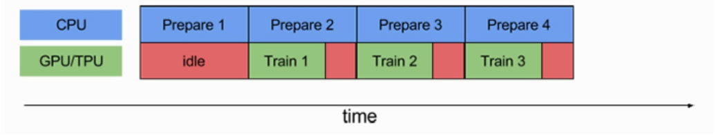
When training the model, we hope to make full use of computing resources and reduce the no-load time of CPU/GPU. However, sometimes, the preparation and processing of data sets is very time-consuming, so we need to spend a lot of time preparing the data to be trained before each training. At this time, GPU can only wait for data without load, resulting in a waste of computing resources.
tf. The Dataset object of data provides us with Dataset Prefetch () method enables us to pre fetch several elements from the Dataset object Dataset during training, so that the CPU can prepare data during GPU training, so as to improve the efficiency of the training process
use:
mnist_dataset = mnist_dataset.prefetch(buffer_size=tf.data.experimental.AUTOTUNE)
-
Parameter buffer_size can be set manually or TF data. experimental. Autotune so that TensorFlow automatically selects the appropriate value.
-
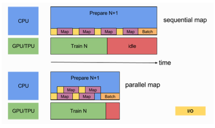
2. There is another way to improve the utilization of CPU resources
- Dataset.map() can also use multi GPU resources to transform data items in parallel, so as to improve efficiency.
By setting dataset Num of map()_ parallel_ The calls parameter implements the parallelization of data conversion. The diagram above shows non parallelization, and the diagram below shows two cores in parallel. The time will be reduced
# Add parameter, num_parallel_calls is set to TF data. experimental. Autotune to let TensorFlow automatically select the appropriate value
train_dataset = train_dataset.map(
        map_func=_decode_and_resize,
        num_parallel_calls=tf.data.experimental.AUTOTUNE)
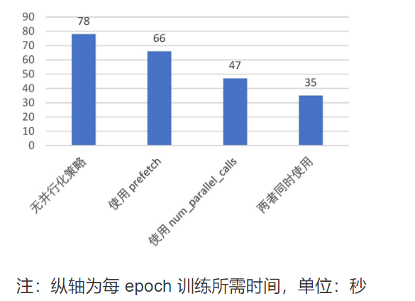
Through the use of prefetch() and adding num in the process of map()_ parallel_ With the call parameter, the training time of the model can be reduced to half or even less.
4.6. Case 5: cat and dog image classification
The data set comes from a competition on kaggle: Dogs vs. Cats , there are 25000 training sets, with half for cats and half for dogs. There are 12500 test sets, and it is not calibrated whether it is a cat or a dog.

- Objective: to take cat and dog picture classification task as an example
- Use TF Data combined with TF IO and TF Image create Dataset dataset
- Datasets can be downloaded here: https://www.floydhub.com/fastai/datasets/cats-vs-dogs
- Steps:
- 1. Acquisition and construction of data sets
- 2. Model building and encapsulation
- 3. Implementation of training and testing process
1. Acquisition and construction of data sets
class CatOrDog(object):
    """Cat dog classification
    """
    num_epochs = 1
    batch_size = 32
    learning_rate = 0.001
        # Training directory
    train_cats_dir = '/root/cv_project/tf_example/cats_vs_dogs/train/cats/'
    train_dogs_dir = '/root/cv_project/tf_example/cats_vs_dogs/train/dogs/'
    # Verify directory
    test_cats_dir = '/root/cv_project/tf_example/cats_vs_dogs/valid/cats/'
    test_dogs_dir = '/root/cv_project/tf_example/cats_vs_dogs/valid/dogs/'

    def __init__(self):
        # 1. Read the cat and dog file of the training set
        self.train_cat_filenames = tf.constant([CatOrDog.train_cats_dir + filename
                                                for filename in os.listdir(CatOrDog.train_cats_dir)])
        self.train_dog_filenames = tf.constant([CatOrDog.train_dogs_dir + filename
                                                for filename in os.listdir(CatOrDog.train_dogs_dir)])
        # 2. Merge the cat and dog file list, and initialize the target value of cat and dog. 0 is cat and 1 is dog
        self.train_filenames = tf.concat([self.train_cat_filenames, self.train_dog_filenames], axis=-1)
        self.train_labels = tf.concat([
            tf.zeros(self.train_cat_filenames.shape, dtype=tf.int32),
            tf.ones(self.train_dog_filenames.shape, dtype=tf.int32)],
            axis=-1)
Define the data acquisition method through TF Data assignment
    def get_batch(self):
        """obtain dataset batch data
        :return:
        """
        train_dataset = tf.data.Dataset.from_tensor_slices((self.train_filenames, self.train_labels))
        # map, random, batch and pre storage of data
        train_dataset = train_dataset.map(
            map_func=_decode_and_resize,
            num_parallel_calls=tf.data.experimental.AUTOTUNE)
        train_dataset = train_dataset.shuffle(buffer_size=20000)
        train_dataset = train_dataset.batch(CatOrDog.batch_size)
        train_dataset = train_dataset.prefetch(tf.data.experimental.AUTOTUNE)
        return train_dataset

# Image processing function, read, decode and modify the input shape
def _decode_and_resize(filename, label):
    image_string = tf.io.read_file(filename)
    image_decoded = tf.image.decode_jpeg(image_string)
    image_resized = tf.image.resize(image_decoded, [256, 256]) / 255.0
    return image_resized, label
2. Model building and encapsulation
By constructing a two-layer convolution + two fully connected layers network
        self.model = tf.keras.Sequential([
            tf.keras.layers.Conv2D(32, 3, activation='relu', input_shape=(256, 256, 3)),
            tf.keras.layers.MaxPooling2D(),
            tf.keras.layers.Conv2D(32, 5, activation='relu'),
            tf.keras.layers.MaxPooling2D(),
            tf.keras.layers.Flatten(),
            tf.keras.layers.Dense(64, activation='relu'),
            tf.keras.layers.Dense(2, activation='softmax')
        ])
3. Implementation of training and testing process
In the process of model training, it is unnecessary to specify ckpt and tensorboard callbacks, and you can specify the experiment yourself
    def train(self, train_dataset):
        """Training process
        :return:
        """
        self.model.compile(
            optimizer=tf.keras.optimizers.Adam(learning_rate=CatOrDog.learning_rate),
            loss=tf.keras.losses.sparse_categorical_crossentropy,
            metrics=[tf.keras.metrics.sparse_categorical_accuracy]
        )

        self.model.fit(train_dataset, epochs=CatOrDog.num_epochs)
        self.model.save_weights("./ckpt/cat_or_dogs.h5")
Test process
- 1. You need to provide a dataset for reading test data and
- 2. For model prediction, you can save the model first and then read it again for prediction
    def test(self):

        # 1. Build test dataset
        test_cat_filenames = tf.constant([CatOrDog.test_cats_dir + filename
                                          for filename in os.listdir(CatOrDog.test_cats_dir)])
        test_dog_filenames = tf.constant([CatOrDog.test_dogs_dir + filename
                                          for filename in os.listdir(CatOrDog.test_dogs_dir)])
        test_filenames = tf.concat([test_cat_filenames, test_dog_filenames], axis=-1)
        test_labels = tf.concat([
            tf.zeros(test_cat_filenames.shape, dtype=tf.int32),
            tf.ones(test_dog_filenames.shape, dtype=tf.int32)],
            axis=-1)
                # 2. Build dataset
        test_dataset = tf.data.Dataset.from_tensor_slices((test_filenames, test_labels))
        test_dataset = test_dataset.map(_decode_and_resize)
        test_dataset = test_dataset.batch(batch_size)

        # 3. Load the model for evaluation
        if os.path.exists("./ckpt/cat_or_dogs.h5"):
            self.model.load_weights("./ckpt/cat_or_dogs.h5")

        print(self.model.metrics_names)
        print(self.model.evaluate(test_dataset))
4.6. 6 Introduction to imagedatagenerator
When there are a large number of local images, we need to generate tensor image data batches through real-time data enhancement. The data will continue to cycle (by batch). Here is a powerful tool
1. Read local pictures and categories during training
tf.keras.preprocessing.image.ImageDataGenerator(featurewise_center=False,
                                             samplewise_center=False,
                                             featurewise_std_normalization=False,
                                             samplewise_std_normalization=False,
                                             zca_whitening=False,
                                             zca_epsilon=1e-06,
                                             rotation_range=0,
                                             width_shift_range=0.0,
                                             height_shift_range=0.0,
                                             brightness_range=None,
                                             shear_range=0.0,
                                             zoom_range=0.0,
                                             channel_shift_range=0.0,
                                             fill_mode='nearest',
                                             cval=0.0,
                                             horizontal_flip=False,
                                             vertical_flip=False,
                                             rescale=None,
                                             preprocessing_function=None,
                                             data_format=None,
                                             validation_split=0.0,
                                             dtype=None)
-
For complete parameter introduction, please refer to the documents on TensorFlow's official website: https://www.tensorflow.org/api_docs/python/tf/keras/preprocessing/image/ImageDataGenerator#view-aliases
-
train_generator = ImageDataGenerator()
- Produce batch tensor values for pictures and provide data enhancements
- rescale=1.0 / 255,: standardized
- zca_whitening=False: # zca whitening is used to reduce the dimension of the image by PCA and reduce the redundant information of the image
- rotation_range=20: the default is 0, the rotation angle. A value is randomly generated in this angle range
- width_shift_range=0.2, default: 0, horizontal translation
- height_shift_range=0.2: default 0, vertical translation
- shear_range=0.2: # translation transformation
- zoom_range=0.2:
- horizontal_flip=True: flip horizontally
2. Introduction to use method
- Use flow(x, y, batch_size)
(x_train, y_train), (x_test, y_test) = cifar10.load_data()

datagen = ImageDataGenerator(
        featurewise_center=True,
        featurewise_std_normalization=True,
        rotation_range=20,
        width_shift_range=0.2,
        height_shift_range=0.2,
        horizontal_flip=True)

for e in range(epochs):
        print('Epoch', e)
        batches = 0
        for x_batch, y_batch in datagen.flow(x_train, y_train, batch_size=32):
            model.fit(x_batch, y_batch)
-
Using train_generator.flow_from_directory(
-
directory=path, # read directory
-
target_size=(h,w), # target shape
-
batch_size=size, # batch quantity
-
class_mode='binary ', # target value format, one of "category", "binary", "sparse",
- "categorical" : 2D one-hot encoded labels
- "binary" will be 1D binary labels
-
shuffle=True
-
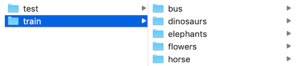
This API fixes the format of the read directory. Refer to:
-
data/
    train/
        dogs/
            dog001.jpg
            dog002.jpg
            ...
        cats/
            cat001.jpg
            cat002.jpg
            ...
    validation/
        dogs/
            dog001.jpg
            dog002.jpg
            ...
        cats/
            cat001.jpg
            cat002.jpg
            ...
-
4.6. Case 7: combination of ImageDataGenerator and migration learning (based on VGG)
4.6. 7.1 case effect
Epoch 1/2
 1/13 [=>............................] - ETA: 3:20 - loss: 1.6811 - acc: 0.1562
 2/13 [===>..........................] - ETA: 3:01 - loss: 1.5769 - acc: 0.2500
 3/13 [=====>........................] - ETA: 2:44 - loss: 1.4728 - acc: 0.3958
 4/13 [========>.....................] - ETA: 2:27 - loss: 1.3843 - acc: 0.4531
 5/13 [==========>...................] - ETA: 2:14 - loss: 1.3045 - acc: 0.4938
 6/13 [============>.................] - ETA: 1:58 - loss: 1.2557 - acc: 0.5156
 7/13 [===============>..............] - ETA: 1:33 - loss: 1.1790 - acc: 0.5759
 8/13 [=================>............] - ETA: 1:18 - loss: 1.1153 - acc: 0.6211
 9/13 [===================>..........] - ETA: 1:02 - loss: 1.0567 - acc: 0.6562
10/13 [======================>.......] - ETA: 46s - loss: 1.0043 - acc: 0.6875
11/13 [========================>.....] - ETA: 31s - loss: 0.9580 - acc: 0.7159
12/13 [==========================>...] - ETA: 15s - loss: 0.9146 - acc: 0.7344
13/13 [==============================] - 249s 19s/step - loss: 0.8743 - acc: 0.7519 - val_loss: 0.3906 - val_acc: 0.9000
Epoch 2/2
 1/13 [=>............................] - ETA: 2:56 - loss: 0.3862 - acc: 1.0000
 2/13 [===>..........................] - ETA: 2:44 - loss: 0.3019 - acc: 1.0000
 3/13 [=====>........................] - ETA: 2:35 - loss: 0.2613 - acc: 1.0000
 4/13 [========>.....................] - ETA: 2:01 - loss: 0.2419 - acc: 0.9844
 5/13 [==========>...................] - ETA: 1:49 - loss: 0.2644 - acc: 0.9688
 6/13 [============>.................] - ETA: 1:36 - loss: 0.2494 - acc: 0.9688
 7/13 [===============>..............] - ETA: 1:24 - loss: 0.2362 - acc: 0.9732
 8/13 [=================>............] - ETA: 1:10 - loss: 0.2234 - acc: 0.9766
 9/13 [===================>..........] - ETA: 58s - loss: 0.2154 - acc: 0.9757
10/13 [======================>.......] - ETA: 44s - loss: 0.2062 - acc: 0.9781
11/13 [========================>.....] - ETA: 29s - loss: 0.2007 - acc: 0.9801
12/13 [==========================>...] - ETA: 14s - loss: 0.1990 - acc: 0.9792


13/13 [==============================] - 243s 19s/step - loss: 0.1923 - acc: 0.9809 - val_loss: 0.1929 - val_acc: 0.9300
4.6. 7.2 data sets and migration requirements
Data set is the recognition of 5 categories of pictures in a scene
We use the existing VGG model to fine tune
4.6. 7.3 ideas and steps
- Read local picture data and categories
- keras. preprocessing. The image import imagedatagenerator provides read conversion capabilities
- Structure modification of the model (add our own classification layer)
- freeze out the original VGG model
- How to compile, train and save models
- Input data for prediction
4.6. 7.4 read local pictures and categories during training
- Read code based on the above tool
train_datagen = ImageDataGenerator(
            rescale=1./255,
            shear_range=0.2,
            zoom_range=0.2,
            horizontal_flip=True)

test_datagen = ImageDataGenerator(rescale=1./255)

train_generator = train_datagen.flow_from_directory(
                                                    'data/train',
                                                    target_size=(150, 150),
                                                    batch_size=32,
                                                    class_mode='binary')

validation_generator = test_datagen.flow_from_directory(
                                                        'data/validation',
                                                        target_size=(150, 150),
                                                        batch_size=32,
                                                        class_mode='binary')
# Using fit_generator
model.fit_generator(
train_generator,
steps_per_epoch=2000,
epochs=50,
validation_data=validation_generator,
validation_steps=800)
code:
Import package first
import tensorflow as tf
from tensorflow import keras
from tensorflow.python.keras.preprocessing.image import ImageDataGenerator
We define a class for migration learning, and then set the relevant properties and read the code
class TransferModel(object):

    def __init__(self):

        self.model_size = (224, 224)
        self.train_dir = "./data/train/"
        self.test_dir = "./data/test/"
        self.batch_size = 32

        self.train_generator = ImageDataGenerator(rescale=1.0 / 255)
        self.test_generator = ImageDataGenerator(rescale=1.0 / 255)

    def read_img_to_generator(self):
        """
        Read local fixed format data
        :return:
        """
        train_gen = self.train_generator.flow_from_directory(directory=self.train_dir,
                                                             target_size=self.model_size,
                                                             batch_size=self.batch_size,
                                                             class_mode='binary',
                                                             shuffle=True)
        test_gen = self.test_generator.flow_from_directory(directory=self.test_dir,
                                                           target_size=self.model_size,
                                                           batch_size=self.batch_size,
                                                           class_mode='binary',
                                                           shuffle=True)
        return train_gen, test_gen
The print result is
<keras_preprocessing.image.DirectoryIterator object at 0x12f52cf28>
4.6. 7.5 modification of VGg model and addition of full connection layer - GlobalAveragePooling2D
- notop model:
- Whether it includes the last three fully connected layers at the top of the network. It is used for fine tuning and specially open source this kind of model.
'weights='imagenet', which means the weight of VGG's pre training in Imagenet competition. Use resnet training
# In__ init__ Add in
self.base_model = VGG16(weights='imagenet', include_top=False)
base_ The model will have relevant attributes, the input structure of the model: inputs, the output structure of the model. We need to get the input of the existing VGG and the output of the user-defined model to build a new model.
Model source code:
    if include_top:
        # Classification block
        x = layers.Flatten(name='flatten')(x)
        x = layers.Dense(4096, activation='relu', name='fc1')(x)
        x = layers.Dense(4096, activation='relu', name='fc2')(x)
        x = layers.Dense(classes, activation='softmax', name='predictions')(x)
    else:
        if pooling == 'avg':
            x = layers.GlobalAveragePooling2D()(x)
        elif pooling == 'max':
            x = layers.GlobalMaxPooling2D()(x)
- One GlobalAveragePooling2D + two fully connected layers
- In the image classification task, the size of the model after passing through the last CNN layer is [bath_size, img_width, img_height, channels]. The usual method is: connect a flat layer, change the size to [batch_size, w_channels], and then connect at least one FC layer. The biggest problem in this way is that there are many model parameters and it is easy to over fit.
- Use the pooling layer to replace the last FC layer
The explanation is as follows:
from keras.layers import Dense, Input, Conv2D
from keras.layers import MaxPooling2D, GlobalAveragePooling2D

x = Input(shape=[8, 8, 2048])
# Assume that the layer output of the last CNN layer is (None, 8, 8, 2048)
x = GlobalAveragePooling2D(name='avg_pool')(x)  # shape=(?, 2048)
# The average value of each characteristic graph is taken as the output to replace the full connection layer
x = Dense(1000, activation='softmax', name='predictions')(x)  # shape=(?, 1000)
# 1000 is the category
- Category 5 picture recognition model modification
We need to get the basic VGG model, and VGG provides trained models with all layer parameters and notop models without full connection layer parameters
from tensorflow.python.keras import Model
def refine_vgg_model(self):
    """
        Add tail full connection layer
        :return:
        """
    # [<tf.Tensor 'block5_pool/MaxPool:0' shape=(?, ?, ?, 512) dtype=float32>]
    x = self.base_model.outputs[0]

    # Output to the full connection layer, plus global pooling [none,?,?, 512] - > [none, 1 * 512]
    x = keras.layers.GlobalAveragePooling2D()(x)
    x = keras.layers.Dense(1024, activation=tf.nn.relu)(x)
    y_predict = keras.layers.Dense(5, activation=tf.nn.softmax)(x)

    model = keras.Model(inputs=self.base_model.inputs, outputs=y_predict)

    return model
4.6. 7.6 structure of freeze VGg model
Objective: let the weight parameters in VGG structure not participate in the training, but only the weight parameters of the last two layers of fully connected network we added
- By using the layer of each layer trainable=False
    def freeze_vgg_model(self):
        """
        freeze fall VGG Structure of
        :return:
        """
        for layer in self.base_model.layers:
            layer.trainable = False
4.6. 7.7 compilation and training
- compile
It is also compiled. In the transfer learning algorithm, the learning rate initializes small values, 0.001,0.0001. Because it has been updated on the basis of the trained model, it does not need too much learning rate to learn
    def compile(self, model):

        model.compile(optimizer=keras.optimizers.Adam(),
                      loss=keras.losses.sparse_categorical_crossentropy,
                      metrics=['accuracy'])
- main function
if __name__ == '__main__':
    tm = TransferModel()

    train_gen, test_gen = tm.read_img_to_generator()
    model = tm.refine_vgg_model()

    tm.freeze_vgg_model()
    tm.compile(model)
    tm.fit(model, train_gen, test_gen)
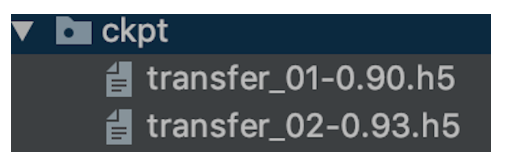
4.6. 7.8 forecasting
The prediction step is to read the picture, process it into the model, and load our trained model
    def predict(self, model):

        model.load_weights("./Transfer.h5")

        # 2. Load and type modify pictures
        image = load_img("./data/test/dinosaurs/402.jpg", target_size=(224, 224))

        print(image)
        # Convert to numpy array array
        image = img_to_array(image)
        print("Shape of picture:", image.shape)

        # Shape changed from 3 dimensions to 4 dimensions
        img = image.reshape((1, image.shape[0], image.shape[1], image.shape[2]))
        print("Change shape result:", img.shape)

        # 3. Processing image content, normalization processing, etc. for prediction
        img = preprocess_input(img)
        print(img.shape)
        y_predict = model.predict(img)

        index = np.argmax(y_predict, axis=1)

        print(self.label_dict[str(index[0])])
Create a dictionary of picture categories
self.label_dict = {
            '0': 'bus',
            '1': 'dinosaurs',
            '2': 'elephants',
            '3': 'flowers',
            '4': 'horse'
        }
4.6. 6 Summary
- Checkpoint usage
- TensorBoard use
- tf.data module usage
- Use of ImageDataGenerator
keras_tool.py
import tensorflow as tf
import numpy as np
import os
os.environ["TF_CPP_MIN_LOG_LEVEL"] = "2"


def function_tool():

    (train_data, train_label), (_, _) = tf.keras.datasets.mnist.load_data()
    # [60000, 28, 28, 1]
    train_data = np.expand_dims(train_data.astype(np.float32) / 255.0, axis=-1)
    mnist_dataset = tf.data.Dataset.from_tensor_slices((train_data, train_label))

    # 1. Flip processing
    def rot90(image, label):
        image = tf.image.rot90(image)
        return image, label

    mnist_dataset = mnist_dataset.map(rot90)
    mnist_dataset = mnist_dataset.batch(4)

    for images, labels in mnist_dataset:
        print(labels.numpy())
        print(images)


def _decode_and_resize(filename, label):
    """For the entered datset Analyze the pictures in
    :param filename: Picture full path
    :param label: target value
    :return:
    """
    image_string = tf.io.read_file(filename)
    image_decoded = tf.image.decode_jpeg(image_string)
    image_resized = tf.image.resize(image_decoded, [256, 256]) / 255.0
    return image_resized, label


# 1. Acquisition and construction of data sets
# 2. Model building and encapsulation
# 3. Implementation of training and testing process
class CatOrDog(object):
    """Cat and dog classification, case, use tf.data Read data
    """
    num_epochs = 1
    batch_size = 32
    learning_rate = 0.001
    # Training directory
    train_cats_dir = '/root/cv_project/tf_example/cats_vs_dogs/train/cats/'
    train_dogs_dir = '/root/cv_project/tf_example/cats_vs_dogs/train/dogs/'
    # Verify directory
    test_cats_dir = '/root/cv_project/tf_example/cats_vs_dogs/valid/cats/'
    test_dogs_dir = '/root/cv_project/tf_example/cats_vs_dogs/valid/dogs/'

    def __init__(self):
        # 1. Acquisition and construction of data sets
        # Read the file name in the directory and merge the cat and dog files
        self.train_cat_filenames = tf.constant([CatOrDog.train_cats_dir + filename for
                                                filename in os.listdir(CatOrDog.train_cats_dir)])
        self.train_dog_filenames = tf.constant([CatOrDog.train_dogs_dir + filename for
                                                filename in os.listdir(CatOrDog.train_dogs_dir)])

        self.train_filenames = tf.concat([self.train_cat_filenames, self.train_dog_filenames], axis=-1)
        # Construct the target value results of cat 0 and dog 1
        self.train_labels = tf.concat([tf.zeros(self.train_cat_filenames.shape, dtype=tf.int32),
                                      tf.ones(self.train_dog_filenames.shape, dtype=tf.int32)],
                                      axis=-1)

        self.model = tf.keras.Sequential([
            tf.keras.layers.Conv2D(32, 3, activation='relu', input_shape=(256, 256, 3)),
            tf.keras.layers.MaxPooling2D(),
            tf.keras.layers.Conv2D(32, 5, activation='relu'),
            tf.keras.layers.MaxPooling2D(),
            tf.keras.layers.Flatten(),
            tf.keras.layers.Dense(64, activation='relu'),
            tf.keras.layers.Dense(2, activation='softmax')
        ])

    def get_batch(self):
        """obtain dataset Type of training data process
        :return:
        """
        # from_tensor_slices
        train_dataset = tf.data.Dataset.from_tensor_slices((self.train_filenames, self.train_labels))
        # map, shuffle, batch, prefetch
        train_dataset = train_dataset.map(_decode_and_resize)
        train_dataset = train_dataset.shuffle(buffer_size=20000)
        train_dataset = train_dataset.batch(CatOrDog.batch_size)
        train_dataset = train_dataset.repeat(1)
        train_dataset = train_dataset.prefetch(tf.data.experimental.AUTOTUNE)
        return train_dataset

    def train(self, train_dataset):
        """Training process
        :return:
        """
        self.model.compile(
            optimizer=tf.keras.optimizers.Adam(learning_rate=CatOrDog.learning_rate),
            loss=tf.keras.losses.sparse_categorical_crossentropy,
            metrics=[tf.keras.metrics.sparse_categorical_accuracy]
        )

        self.model.fit(train_dataset)
        self.model.save_weights("./ckpt/cat_or_dogs.h5")

    def test(self):
        # 1. Build test dataset
        test_cat_filenames = tf.constant([CatOrDog.test_cats_dir + filename
                                          for filename in os.listdir(CatOrDog.test_cats_dir)])
        test_dog_filenames = tf.constant([CatOrDog.test_dogs_dir + filename
                                          for filename in os.listdir(CatOrDog.test_dogs_dir)])
        test_filenames = tf.concat([test_cat_filenames, test_dog_filenames], axis=-1)
        test_labels = tf.concat([
            tf.zeros(test_cat_filenames.shape, dtype=tf.int32),
            tf.ones(test_dog_filenames.shape, dtype=tf.int32)],
            axis=-1)
        # 2. Build dataset
        test_dataset = tf.data.Dataset.from_tensor_slices((test_filenames, test_labels))
        test_dataset = test_dataset.map(_decode_and_resize)
        test_dataset = test_dataset.batch(CatOrDog.batch_size)

        # 3. Load the model for evaluation
        if os.path.exists("./ckpt/cat_or_dogs.h5"):
            self.model.load_weights("./ckpt/cat_or_dogs.h5")

        print(self.model.metrics_names)
        print(self.model.evaluate(test_dataset))


if __name__ == '__main__':
    # function_tool()
    cod = CatOrDog()
    train_dataset = cod.get_batch()
    print(train_dataset)
    # cod.train(train_dataset)
    cod.test_v2()
tfrecords_example.py
import os
import tensorflow as tf
import os
os.environ["TF_CPP_MIN_LOG_LEVEL"] = "2"

train_cats_dir = './cats_vs_dogs/train/cats/'
train_dogs_dir = './cats_vs_dogs/train/dogs/'
tfrecord_file = './cats_vs_dogs/train.tfrecords'


def main():

    train_cat_filenames = [train_cats_dir + filename for filename in os.listdir(train_cats_dir)]
    train_dog_filenames = [train_dogs_dir + filename for filename in os.listdir(train_dogs_dir)]
    train_filenames = train_cat_filenames + train_dog_filenames
    # Set the tag of cat class to 0 and the tag of dog class to 1
    train_labels = [0] * len(train_cat_filenames) + [1] * len(train_dog_filenames)

    with tf.io.TFRecordWriter(tfrecord_file) as writer:
        for filename, label in zip(train_filenames, train_labels):
            # 1. Read the dataset picture to memory, and the image is a Byte type string
            image = open(filename, 'rb').read()
            # 2. Establish TF train. Feature dictionary
            feature = {
                'image': tf.train.Feature(bytes_list=tf.train.BytesList(value=[image])),  # The picture is a Bytes object
                'label': tf.train.Feature(int64_list=tf.train.Int64List(value=[label]))  # The label is an Int object
            }
            # 3. Create an Example from a dictionary
            example = tf.train.Example(features=tf.train.Features(feature=feature))
            # 4 \ serialize Example and write it to TFRecord file
            writer.write(example.SerializeToString())


def read():

    # 1. Read TFRecord file
    raw_dataset = tf.data.TFRecordDataset(tfrecord_file)

    # 2. Define the Feature structure and tell the decoder what the type of each Feature is
    feature_description = {
        'image': tf.io.FixedLenFeature([], tf.string),
        'label': tf.io.FixedLenFeature([], tf.int64),
    }

    # 3. Serialize each TF in the TFRecord file train. Example decoding
    def _parse_example(example_string):
        feature_dict = tf.io.parse_single_example(example_string, feature_description)
        feature_dict['image'] = tf.io.decode_jpeg(feature_dict['image'])  # Decoding JPEG pictures
        return feature_dict['image'], feature_dict['label']

    dataset = raw_dataset.map(_parse_example)

    for image, label in dataset:
        print(image, label)


if __name__ == '__main__':
    # main()
    read()
model_serving.py
import tensorflow as tf
import os
os.environ["TF_CPP_MIN_LOG_LEVEL"] = "2"


def main():
    num_epochs = 1
    batch_size = 32
    learning_rate = 0.001

    model = tf.keras.models.Sequential([
        tf.keras.layers.Flatten(),
        tf.keras.layers.Dense(120, activation=tf.nn.relu),
        tf.keras.layers.Dense(100),
        tf.keras.layers.Softmax()
    ])

    (train, train_label), (test, test_label) = \
                tf.keras.datasets.cifar100.load_data()

    model.compile(
        optimizer=tf.keras.optimizers.Adam(learning_rate=learning_rate),
        loss=tf.keras.losses.sparse_categorical_crossentropy,
        metrics=[tf.keras.metrics.sparse_categorical_accuracy]
    )
    model.fit(train, train_label, epochs=num_epochs, batch_size=batch_size)

    tf.saved_model.save(model, "./saved/mlp/2")


def test():

    model = tf.saved_model.load("./saved/mlp/2")

    (_, _), (test, test_label) = \
        tf.keras.datasets.cifar100.load_data()

    y_predict = model(test)

    sparse_categorical_accuracy = tf.keras.metrics.SparseCategoricalAccuracy()
    sparse_categorical_accuracy.update_state(y_true=test_label, y_pred=y_predict)
    print("The accuracy of the test set is: %f" % sparse_categorical_accuracy.result())


def client():
    import json
    import numpy as np
    import requests

    (_, _), (test, test_label) = \
        tf.keras.datasets.cifar100.load_data()

    # 1. Constructed request
    data = json.dumps({"instances": test[:10].tolist()})
    headers = {"content-type": "application/json"}

    json_response = requests.post('http://localhost:8501/v1/models/mlp:predict',
                                  data=data, headers=headers)

    predictions = np.array(json.loads(json_response.text)['predictions'])
    print(predictions)
    print(np.argmax(predictions, axis=-1))
    print(test_label[:10])


if __name__ == '__main__':
    # main()
    # test()
    client()