Another widely used model reuse method is fine tuning, which complements feature extraction. For the frozen model base used for feature extraction, fine tuning refers to "thawing" the top layers, and jointly training the thawed layers with the newly added part (in this case, the fully connected classifier). It is called fine tuning because it only slightly adjusts the more abstract representations in the reused model to make them more relevant to the problem at hand.

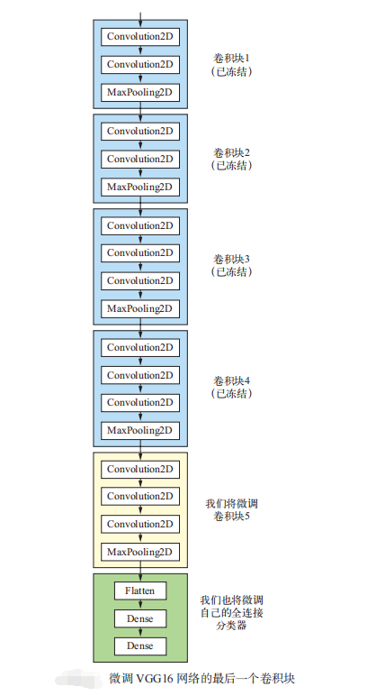
As mentioned earlier, the convolution basis of VGG16 is frozen in order to train a randomly initialized classifier on it. Similarly, only when the above classifier has been trained can the top layers of convolution basis be fine tuned. If the classifier is not well trained, the error signal transmitted through the network during training will be particularly large, and the representations learned before the fine-tuning layers will be destroyed. Therefore, the steps to fine tune the network are as follows.

1. Add a custom network to the trained base network.
2. Freeze the network base.
3. The part added to the training.
4. Thaw some layers of the base network.
5. Joint training thawed these layers and added parts.

Why not fine tune more layers? Why not fine tune the entire convolution basis?

1. The layer closer to the bottom of the convolution base encodes more general reusable features, while the layer closer to the top encodes more specialized features. Fine tuning these more specialized features is more useful because they need to change purpose on your new problem. Fine tuning the layer closer to the bottom will get less return.
2. The more training parameters, the greater the risk of over fitting. The convolution basis has 15 million parameters, so training so many parameters on your small data set is risky.
   The training code of fine tuning model is as follows:

from tensorflow.keras.preprocessing.image import ImageDataGenerator
from PIL import Image
from tensorflow.keras import layers
from tensorflow.keras import models
from tensorflow.keras import optimizers
import matplotlib.pyplot as plt
from tensorflow.keras.preprocessing import image as kimage
from tensorflow.keras.applications import VGG16
import numpy as np

'''
ImageDataGenerator Image data reading can be completed
 Read image file
 take jpeg Image decoded as RGB Pixel network
 Convert these pixels to floating-point tensors and scale them to floating-point tensors~1 between
'''
#Catalog of training samples
train_dir='./dataset/training_set/'
#Catalog of validation samples
validation_dir='./dataset/validation_set/'
#Test sample catalog
test_dir='./dataset/test_set/'

#Training sample generator
#Note that data enhancement can only be used for training data, not for verification data and test data
'''
Data enhancement
'''
#Set data enhancement
'''
rotation_range Is the angle value (at 0~180 Range), indicating the angle range of random rotation of the image.
width_shift and height_shift Is the range (relative to the total width) in which the image is translated horizontally or vertically
 Degree or proportion of total height).
shear_range Is the angle of the random staggered transformation.
zoom_range Is the range of random scaling of the image.
horizontal_flip Is to flip half the image horizontally at random. If there is no assumption of horizontal asymmetry (such as true)
Images of the real world), this approach is meaningful.
fill_mode Is the method used to fill in newly created pixels, which may come from rotation or width/Height translation.
'''
train_datagen=ImageDataGenerator(
    rescale=1./255,
    rotation_range=40,
    width_shift_range=0.2,
    height_shift_range=0.2,
    shear_range=0.2,
    zoom_range=0.2,
    horizontal_flip=True,
    fill_mode='nearest')

train_generator=train_datagen.flow_from_directory(
    directory=train_dir,
    target_size=(150,150),
    class_mode='binary',
    batch_size=20
)

#Validation sample generator
validation_datagen=ImageDataGenerator(rescale=1./255)
validation_generator=train_datagen.flow_from_directory(
    directory=validation_dir,
    target_size=(150,150),
    class_mode='binary',
    batch_size=20
)

#Test sample generator
test_datagen=ImageDataGenerator(rescale=1./255)
test_generator=train_datagen.flow_from_directory(
    directory=test_dir,
    target_size=(150,150),
    class_mode='binary',
    batch_size=20
)



if __name__=='__main__':
    conv_base=VGG16(weights='imagenet',
                include_top=False,
                input_shape=(150,150,3))
    #Freeze the convolution basis to ensure that its weight remains unchanged in the training process
    conv_base.trainable=False
    #Build training network
    model=models.Sequential()
    model.add(conv_base)
    model.add(layers.Flatten())
    model.add(layers.Dense(units=256,activation='relu'))
    model.add(layers.Dense(units=1,activation='sigmoid'))

    model.compile(optimizer=optimizers.RMSprop(learning_rate=1e-4),
                  loss='binary_crossentropy',
                  metrics=['acc'])

    model.summary()

    # The convolution basis of the network is fitted for the first time, and all the classification parts added by the training are frozen
    model.fit_generator(
        train_generator,
        steps_per_epoch=100,
        epochs=30,
        validation_data=validation_generator,
        validation_steps=50
    )

    #Accuracy of test set
    test_eval=model.evaluate_generator(test_generator)
    print(test_eval)

    #Thawing some layers in convolution basis
    conv_base.trainable=True
    for layer in conv_base.layers:
        layer.trainable=False
        if layer.name=='block5_conv1':
            break
    
    for layer in conv_base.layers:
        print(layer.name+':'+str(layer.trainable))

    model.compile(loss='binary_crossentropy',
                  optimizer=optimizers.RMSprop(lr=1e-5),
                  metrics=['acc'])
    # Second fitting network convolution basis partial thawing training thawing part 
    history=model.fit_generator(
        train_generator,
        steps_per_epoch=100,
        epochs=30,
        validation_data=validation_generator,
        validation_steps=50
    )
    test_eval=model.evaluate_generator(test_generator)
    print(test_eval)

    acc = history.history['acc']
    val_acc = history.history['val_acc']
    loss = history.history['loss']
    val_loss = history.history['val_loss']
    epochs = range(1, len(acc) + 1)
    plt.plot(epochs, acc, 'bo', label='Training acc')
    plt.plot(epochs, val_acc, 'b', label='Validation acc')
    plt.title('Training and validation accuracy')
    plt.legend()
    plt.figure()
    plt.plot(epochs, loss, 'bo', label='Training loss')
    plt.plot(epochs, val_loss, 'b', label='Validation loss')
    plt.title('Training and validation loss')
    plt.legend()
    plt.show()

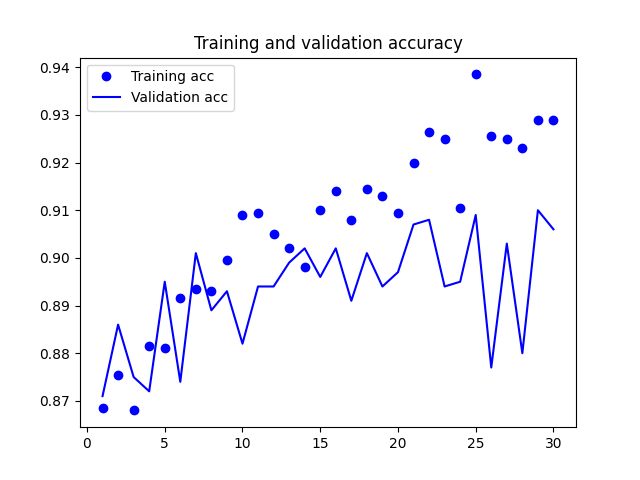
The accuracy curve during model training is shown in the figure below:

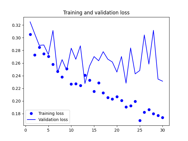
The loss function curve during model training is shown in the figure below: